Geography 291: Geospatial Analysis with Desktop GIS

Chapter 7

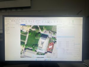
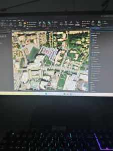
Chapter 7 walks the user through the process of managing a map that contains real imagery. I found this to be a valuable chapter and relatively easy to understand. It taught me how to rotate and move polygons to match the satellite images, as well as create different polygons for new features. The chapter also began to familiarize me with the Edit ribbon, which I feel as though I had not interacted with much in prior chapters. The edit ribbon contained the move and edit vertices buttons. The edit vertices buttons allowed me to add and move vertices to morph a polygon to match the satellite image. There were other ways to edit polygons, though, such as the trace and split buttons. The trace button allowed me to create a selection using the streetpaths as a guide, while the split button allowed me to make two separate polygons out of a single polygon. I had some trouble with the last tutorial of the chapter when asked to import data for a building polygon. I will say that this chapter seemed to easily explain how to change the visual features of a map when needed, which I feel will be quite helpful when building my own maps. 

Chapter 8

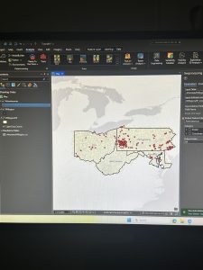
Chapter 8 was shockingly short, with a heavy emphasis on zipcodes and other floating techniques. One technique is the geocode addresses tool, which helps to create dot plots on a map using specific zipcode data. There is also a tool called a collect events tool that does something similar, placing dots, this time with a greater variety of dot sizes. Much of the chapter was a simple walkthrough of different tools, with almost all of them adding or altering points on the map in some way. I find this valuable as it is important to strategize what the most effective way to visualize your data is, and the creators of the GIS platform recognize this by providing the user with many different ways to do this. Additionally, there was some more use of the attribute tables, which is always a good thing to refresh my mind on. I was a bit surprised that ZIP code data points had been covered so late into the textbook, as I would think that this is a form of data that I will be utilizing relatively frequently going forward in my work with the GIS platform. 

Chapter 9

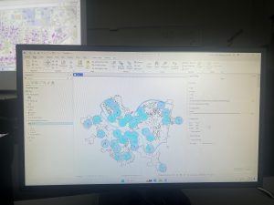
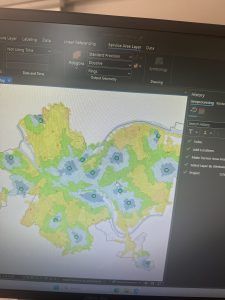
A large aspect of Chapter 9 was to create different types of buffers around different data points on the map. It walked me through how to change the radius of the buffer and what tool to use to create a buffer, which were the pairwise buffer and the multiple ring buffer. The pairwise buffer tool creates a standard radius around the data point, while the multiple ring buffer can create a greater number of buffers, and also provides the option of making them overlap. A lot more was done in the analysis tab within this chapter as well. One of the features from the analysis tab is the service area option, which can change the visual attributes of the data measured within the map. I personally thought that was a cool feature to introduce, and it was interesting to see how different layers of data can be shown in that way. It was also a good way to show how the data can change depending on the distance from a particular point. Another important topic covered within the chapter was the visualization of data in the sense of creating different types of representations, such as tables and dot plots. It felt very appropriate to finish the tutorials off with some additional support in creating tables and such. 

Chapter 7: This chapter was pretty easy and went well for the most part. I ran into an issue in the first tutorial where I could not select the outlines of buildings, but after resetting I was able to complete the tutorial without issue. I encountered no other problems with this chapter.

Chapter 8: Didn’t have any issues with the tutorials for this chapter, the only thing that went wrong was in the second tutorial the computer froze while running the geocoding addresses tool. I waited several minutes for it to unfreeze but ultimately had to power off the computer and restart the tutorial. Afterward, I encountered no issues in this chapter.

Chapter 9: I only had to restart tutorial 3 in this chapter due to making a mistake early on, I think it was with the spatial join tool. Other than that, there were no issues in this chapter. I feel like after completing all these tutorials I am getting a better understanding of how tools work and what they can be used for.

Chapter 1:

Starting with a completed map and working backwards is an interesting tactic to teach beginners how the system works. That way the maps are already mostly constructed and the learning is very specific/ centered in a certain task within that map. Connecting to that, the “Your Turn” sections of the book is a smart way to ensure the reader is actually grasping the material. It makes you use your own brain to work through what was just done as a tutorial on your own. Also, the textbook including photo examples alongside the tutorial is very helpful in making sure I haven’t messed something up. It’s a good visual guideline. On the contents pane, the way it’s arranged to be from what’s drawn first and “on the bottom of everything” makes a lot of sense in regards to a map and layering. I knew everything had its own layer from reading the earlier chapters, but the tutorial extended that thought even further by having this particular overlay. It makes a lot of sense to me that the layers are drawn on top of one another, it’s almost like altering a physical map by adding marks directly on top  of the paper.

A personal connection to the system of GIS that I had thought about when working was the shortcuts. Taking “snapshots” and using Ctrl S to save the project is something I’ve instinctually been drawn to do after spending years working in Photoshop with a similar shortcut interface. I never wanted to lose work, and from that I learned to always save my work, which I’ve found really carries over to this system as well. By having an original base saved/ snapshotted, it lowers the impact a mistake might have on the project, ensuring there is always that beginning point to return to if needed.

Finally, I had a slight moment of frustration at the end of the tutorial when it came to the labeling. The program is such a large system, and it has a crazy amount of buttons, so simply locating where all the different buttons and options are was a lot to process. It was frustrating when I couldn’t figure out where something was hiding in the interface.

 

Chapter 2:

This chapter diverged from the 2D maps, into adjusting them to be seen as a more prominent 3D. I really liked the way that the interpretation of the maps can completely change between 2D and 3D. How some details that may relay a certain type of information isn’t the same linear with the two styles, or how an aspect of the 3D model can bring to light information that couldn’t be seen the other way. This really brings to light the idea of understanding your map. Knowing who/ what the map is for, in order to adjust and label it in a way that will relay the kinds of information needed within its purpose. This chapter really focuses on clarifying the details of the map. By making the subject notable while also adding the necessary context to the background.

Something that I found interesting while working on this chapter, was the mention of color blindness. Which was something I hadn’t actually thought about once when creating all these models of colors. It was neat to see the inclusion of altering how a map is displayed so a person with color blindness could achieve the same aspect of detail when mapping, even without using bunches of colors. It also doubled as a lesson in understanding how to change the symbols of a map, and explaining that a variety of shapes can be used instead of colors to convey the same knowledge of the key.

I will add as a side note, that I absolutely love playing around with the different colors! Obviously the purpose of a map is to convey information, but I find it fun to adjust the colors in an aesthetically pleasing way, or to pair associated colors with the topic of the map.

Chapter 3:

This chapter was interesting because we pivoted even more and went from working within the ArcGIS Pro, to learning the Online system. On that topic, I feel as though in a way, ArcGIS Online is a much smoother/ easier interface to work with. I don’t know exactly how to explain that, but maybe it’s due to the fact that it’s online and available for anyone to access. Perhaps it’s made a bit simpler and cleaner for anyone to play around with and use. Before that section of the tutorial however, I really liked following the detailed explanation of how to create layouts from scratch. This is a very useful skill, in being able to make any style of chart or map view of the project for easy download and display. I liked how the textbook described going about making these layouts. To think about retaining this goal of designing it in a way that anyone could understand it, like you’re sharing the maps to those with no experience in the software. It reminded me of the explanatory mindset of teaching something in a way a child or an alien could grasp.

I have a creative mindset, so I adored the section of the chapter that revolved around storytelling within the StoryMaps. We were giving the map’s their story. In a sense, this is leaning into the analytical aspect of the “Geospatial Analysis.” I appreciated the angle of art, from adding a cover image, to having the potential to completely change the design/ layout. This part, just like creating layouts, is highly important to know how to do. The uses for the completed story and layout are endless. My first thought was using it for a website, or some form of journalism as I thought it resembled an article in a way. It’s returning to the idea in the first textbook of the many everyday uses that GIS has.

The quote from the mathematician, John Tukey, “minimize ink!” is very applicable to mapping on GIS. And I rather enjoyed the idea of never deleting any values even if they don’t add anything to the image. It’s like with art, you might take a hundred photos or create notebooks of sketches, and only a handleful could be things you actually like and will use. You don’t just throw the others out though, because they still hold power in what they don’t show. It’s better to keep something and not use it, then to delete it and realize you really did like it, or did need it after all.

Chapter 7:

This chapter focused on digitizing, which meant that most of it was spent converting various forms of data into forms that work best in ArcGIS. This is super important because there is no universal method of data presentation, and being able to convert and create data of the desired form is crucial for any mapmaking. I was already familiar with many aspects of this chapter from working with other drawing and graphic design apps. I had a lot of fun with it!

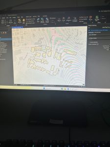
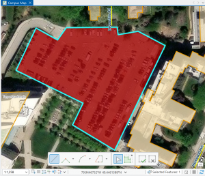
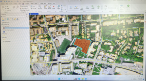
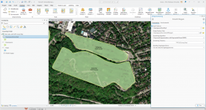
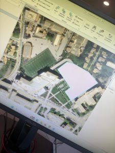
Figure 7.1 Drawing a polygon for the parking lot. 

Creating polygons and using the Trace tool were my favorite parts of this chapter! Honestly, making polygons was easier than I was originally expecting. From the readings earlier in this course, I thought I was going to have to input geographic coordinates to put polygons into the correct spot. I learned that ArcGIS is much kinder and allows you to simply drag and rotate polygons. It’s also very helpful to have a matching basemap or base layers to which you can size your polygons.

Also, I was pleasantly surprised by the capabilities of the Smoothing tool. Once again, I thought there was going to be some sort of complicated algorithm I would have to go through to get a smooth shape, but it’s thankfully just another tool! (I’m sure that the computer performs complicated steps, but I am grateful that I don’t have to do them myself.)

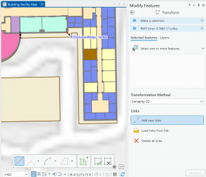
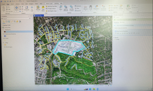
Figure 7.2:  Transforming the SpacePlan layer onto the StudyBldgs layer. 

It took me a few tries to get this right because I attempted to complete this step before looking at the reference photo in the tutorial. At first, I tried drawing an outline around the SpacePlan layer…which definitely did not work. Then, I tried transforming every single vertex, which was unnecessary. (That attempt is shown in the picture above.)

Chapter 8:

This chapter, focused on geocoding, was pretty short. However, there was still a wealth of important techniques and information within! Something that sounded super interesting to me in the beginning of the chapter was the use of Soundex keys to match attribute names (ex. streets) that are not spelled correctly. It seems like a really neat way to code and simplify language. The step I struggled with the most in this chapter was rematching attendee data. For whatever reason, when I tried to click on an individual location, I struggled to find the Match button and successfully rematch the addresses.

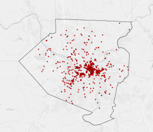
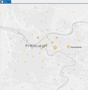
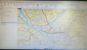
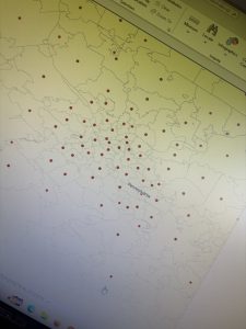
Figure 8.1 Distribution of Attendees using Collect Events tool.

I liked using the Collect Events tool. Being able to turn individual events within certain tracts into collective graduated symbols is a really helpful way to look at the data differently! The concept of match scores is also pretty neat. It’s proof that though the computer is faster at computing than humans, it’s not necessarily smarter. Though the computer does make conjectures and assumptions looking at local context in the data, it doesn’t have the natural reasoning or critical thinking of humans. So yes, mistakes (when inputting addresses, for example) are made by humans in the first place, but then humans go back in after the computer has done its best and apply personal knowledge and community context clues to fill in the gaps.

Chapter 9:

This chapter focused on applying advanced GIS technologies, but thankfully, I found it pretty easy. Tutorial 9-1 introduces the concept of buffers, which I recall reading about in the other text. I find the concept of mapping with buffers really useful and interesting! Buffers are great for determining if objects fall within a certain radius, which is particularly important in fields like public health when determining who may or may not have access to a particular service or facility. 

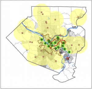
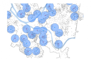
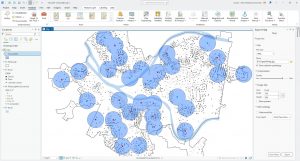
Figure 9.1: 0.5- and 1-mile buffers around public pools in Allegheny County, Pittsburgh.

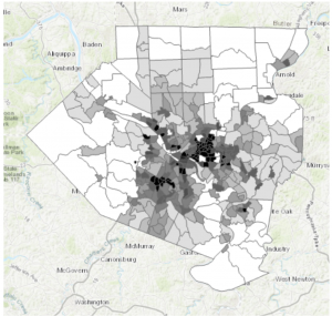
There are 42, 548 youths in the city of Pittsburgh within 1 mile of a pool, which means 87% of youths in Pittsburgh have good accessibility to a pool. (There are 48,903 total youths in Pittsburgh.) In Pittsburgh, 10,718 youth have excellent access to a pool, 20,448 have good access, and 16,264 have fair or poor access. This corresponds to percentages of 22%, 42%, and 33%, respectively. Considering that more youths in Pittsburgh have fair or poor pool access than those with excellent pool access, changes should be made to ensure that more pools can be open for these kids. (Or alternatively, some areas with high pool density can close and those resources can be reallocated to open a pool in an area where it might be the only one.

In Tutorial 9-5, for whatever reason, some of the Cluster IDs were numbered differently, so I had to pay attention while relabeling the features to ensure they matched the data correctly.

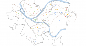
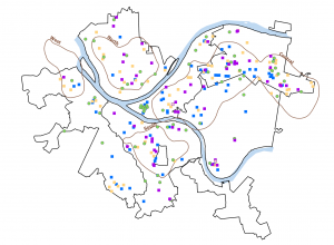
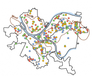
Figure 9.2 Serious Violent Crimes by Age and Gender

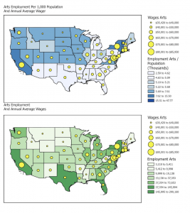
The square shapes correspond to young age groups that committed crimes. The pink and purple shapes are females, and the yellow, green, and blue shapes are males. If I were to take this analysis further, I could impose these features on a streets basemap to determine where they are occurring in terms of area development, or I could create a graduated colors map measuring income to see if more crimes are being committed in lower income areas. 

All of the tutorials are done…hooray! I just want to give a shoutout to the geoprocessing toolbox…absolutely clutch! I would get so excited every time I saw that I could just plug in my inputs and outputs, units of measurement, and queries. Literal lifesaver. 5 stars.

Chapter 7

Chapter 7 was about digitizing, in which I learned how to edit, create, and delete polygon features, create and digitize point features, use cartography tools to smooth features, work with CAD drawings, and spatialy adjust features. I found it very interesting that 7-1 allowed us to edit polygon features on CMU’s campus buildings. I was able to rotate and move existing buildings into a layer, and add vertex points and split polygons to further edit them to match buildings on the world imagery basemap. I found this section to be very fun. I am still a little confused on vertex points and why they are important to use/what the purpose of them are. In 7-2 I was able to create and delete polygon features. I learned that campus planners need polygons of open parking lots for a permeable surface and transportation engineering study.  This section was interesting as I was able to work with parking lots and bus stops.

Section 7-3 was very straightfoward, where I learned about the smooth polygon tool, which is a useful tool to improve the aesthetic or cartorgraphic quality of polygons. I also learned that the features are digitized with just a few line segments and don’t match the true geography. Section 7-4 was the most difficult section, which was about transforming features. I learned about the importance of computer-aided design (CAD). CAD drawings and BIM models use Cartesian coordiantes (which I do not know what it is) and are not geographically referenced to geographic coordinate system, state plane, or Universal Transverse Mercator (UTM) coordinates (which I also do not know what this is). CAD drawings contain layers in one drawing and are color-coded according to the layer color assigned in the CAD drawinsgs. I did not know that you cannot edit CAD drawings directly, and in order to edit it, you have to export the drawing to a feature class after you georeference it to its approximate campus location- and this caused me to be stuck at first.

Chapter 8

Chapter 8 was about geocoding, and I felt as if this was the hardest chapter we have done yet. I have not heard of geocoding prior to this, but I learned that geocoding is a GIS process that matches location fields in tabular data to corresponding fields in existing feature classes, such as TIGER/Line Streets, to map the tabular data. I also learned that a problem with geocoding is that soruce data suppliers and data entry workers can write or type anything they want for an address, including misspellings, abbreviations, omissions, and place-names instead of addresses. I would like to read more and research more about what fuzzy matches and fuzzy methods are- I have heard about this in research articles before and was not too sure what that means. I learned that an algorithim computes a Soundex key, which is a code assigned to names that sound alike, and identifies candidate matches of source and reference street adresses to account for spelling errors.

In 8-1 I geocoded survy data collected by a Pittsburgh arts organization that holds an event each year attended by persons across the country. I found the process of building a zip code locator to be difficult. I’m not too sure what I was doing wrong, but I had a lot of trouble on step 3, as I could not find the locators tab in the catalogs pane. I was alos able to geocode data by zip code. I know the book stated to not select ArcGIS World Geocoding Service or Esri World Geocoder for Address Locater, however I am very interested in these two software systems and what they entail. 8-2 was interesting as I was able to geocode street addresses. It was very interesting to geocode attendee data by street address and select minimum candidate and matching scores, as this has broader implications to public health initatives and outbreak response.

Chapter 9

This chapter was about spatial analysis. I have heard this term being used in the first book we use, and in public health courses, but I have not known what the term means. I learned how to use buffers for proximity analysis. A buffer is a polygon surrounding map features of a feature class. I was able to run the pairwise buffer tool  through buffering Pittsburgh’s 32 public pools to estimate the number of youths ages 5 to 17 that live close, within a half mile, of the nearest pool.  I found 8-1 to be very straight-forward and easy to navigate. I also did do the “your turn” on page 216, which I also was found very easy to change the radius to increase buffer areas. Tutorial 9-2 was about using multiple-ring buffers.  I learned that a multiple-ring buffer for a point looks like a bull’s-eye target, with a central circle and rings extending out.

Furthermore, 9-2 annlowed me to use spatial overaly to get statistics by buffer area. This calculates the percetnage of youths with excellent and good access with the limited number of pools open. I found this was very interesting as the information was already readily available, and it is cool to see the differences between various buffer areas. In tutorial 9-3, I was able to create multiplering service areas for calibrating a gravity model. It was interesting to use service areas to estimate a gravity model of geography that assumes the further apart two features are, the less attraction between them. I did  enjoy making a scatterplot through ArcGIS Pro, as I can see myself utilizing this tool in the future.

 

Ch 7: This chapter focused a lot on how to move, rotate and readjust the shape of certain images. Which reminded me of photoshop and other editing apps used for pictures. In tutorial 7-1., I learned how to move images and make them fit to their corresponding guidelines. At first I struggled with being able to move the selected item, but the book was a great reference to solve my problem. I also struggled with creating polygons in the first part of 7-3., but everything else was fine afterwards. Throughout this chapter, I learned the importance of understanding coordinates and adjusting figures on the GIS maps. Especially when the data is being used to plan or rework an area such as remodeling an old building. Both on the exterior and interior, which is one of the key takeaways I learned from this chapter. For example in tutorial 7-4., I had to analyze the inside space of the Hamburg’s Hall academic building. This activity helped me understand how GIS can be used for interior remodeling or data collection, depending on the research. I believe this is an interesting way to use this technology because it can help architects, engineers or people who use a building to work on ways to improve it. I wonder if this tool is used for any construction or remodeling project on OWU campus. For example, I heard that there is a future solar panel project on campus so I wonder if they used GIS for any planning? Nonetheless, I enjoyed learning how to readjust figures and how GIS can be used for modeling and not just statistical data analysis. This will make the software more fun and interesting to utilize.

Ch 8: This chapter emphasized the tool for geocoding on GIS. I was surprised to see that the introduction was long and how many mistakes have been made with the geocode. One of the major errors of this  process is the misinformation it can create. The introduction mentioned that geocode can interpret misspelled words which can convey inaccurate data. Even though there has been software to solve this problem, it can still be challenging to accurately obtain results. Additionally, I was also surprised to see that this was a short chapter and that there were not a lot of tutorials for geocoding. As the name suggests, these tutorials reminded me a lot about programming because I had to input a lot of information in order to run the feature. In programming, I know that one has to also input specific data and values to obtain the results they want. Another aspect of this tutorial that I noticed was the common use of Pennsylvania as an example. I previously mentioned this in another post, but I am still surprised that New York and Pennsylvania are the main locations we use for these tutorials. I wonder if that was set up so that it would make the data and tutorials easier to understand, or is it just a coincidence? I wonder if in the future tutorials a western state will be mentioned, because I do not recall one being mentioned. Regardless, I enjoyed learning about geocoding and how information learned from the tutorials can be applied on any GIS software.

Ch 9:  Finally, the final chapter of this week’s tutorial focused on spatial analytical methods of the GIS software, such as buffers. This reminded me of a previous tutorial where it also focused on how to create and apply buffers on the software. However, this chapter focused on the different methods of spatial data so the section was broad and less focused on buffers. It was interesting to see how the distance of buffers can visually change the map. For example, in tutorials 9-1., to 9-4., exemplifies how buffers change the map through colors and shapes. Such as in 9-3., where the buffers added color to the map while representing different data in specific areas. This was also used for the other tools such as the data cluster and network analysis to define certain features and areas. I remember that Schuurman described his concern for misinterpreting data from GIS because everyone has a different perspective. Especially if the data does not use a legend to explain the difference between each color. I wonder if some people would prefer aesthetically pleasing visuals on the map instead of practicality. I know some people are more creative than others so would they have a preference on the colors used for representing the data? Perhaps there should be a guideline on how the colors should be interpreted when using GIS. This question may be out of topic, but it was something that I was curious about after following the tutorial and noticing the different colors used. I really enjoyed this week’s tutorial and I hope to keep improving my GIS and technical skills. 

Chapter Six 

 This chapter taught us the Geopreocessing tools. I learned to edit and create polygon features. My favorite part was moving the buildings around. I used CAD drawings to adjust various features. I think the best part of this chapter is that it didn’t feel like I was just following steps, but could see a real purpose. These tools would be great to update maps but also to see how particular features could fit into existing places. For example, if I wanted to look at laying new pathways through the campus, this would be a really helpful way to do it. 

Chapter 8

I practiced geocoding. I learned the main components of geocoding. When reading the introduction to this chapter I learned that there is an algorithm to help with spelling errors. A score is provided when a search is run and has penalty points for problems. This helps to select the best candidate according to what was searched for. This made me wonder if this is how Google Maps looks for the closest match when a misspelling is given. For example I live on County Road 11. Further down the road, the name changes. However, in Google Maps, they suggest the name of the road, further down (actually a different county), as the intended address. It also makes me wonder how this gets corrected. 

Chapter 9

In this chapter I learned how to apply the spatial analysis tools for real world applications. Buffers and multiple-ring buggers are used to measure proximity. I was able to create service areas. I used ArcGis Network Analyst to locate places with constraints and observe patterns. 

Chapter 7:

Chapter seven focuses on creating polygon features, digitize point features, using cartography tools to smooth features, CAD drawings, and spatially adjusting features. Tutorial 7-1 has you edit polygon features to select a specific university building. It has you do this feature to multiple different buildings, with complex shapes and sizes. Into 7-2, the focus is on adding a feature class to polygons. Adding a feature class allows for a select tool along the contents pane that can be clicked on and off for each item you want highlighted. In this chapter it focuses on parking lots. The parking lot highlighted below in red was relatively simple. The only slight issue I had was finding how to make the background color transparent. Into the next steps, it showed us how to remove buildings as the map is updated. One thing I noticed about this specific map was it had been further updated since the book and there was another building still labeled that needed deleted. I went ahead and also deleted that one to get the most accurate map, as well as some more practice. Overall, I have noticed multiple times this semester that many steps are not accurate to the book and the wording has changed, or the map within the software. This has lead to multiple moments of confusion for me using the GIS software. The final step of this tutorial was to outline the main campus portion using snapping. The snapping feature was much easier than the previous selecting, and made the shape much more accurate. This was helpful for the next steps when it had you take the measurements. The next few tutorials were very similar with outlining different buildings and landmarks in different circumstances. This chapter was extremely helpful to learn more about the special features of GIS.

Chapter 8:

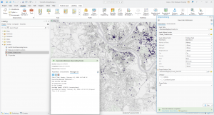
Chapter eight focuses on learning about geocoding. This includes geocoding zip codes and addresses using streets. The tutorial I did for this chapter was 8-1, however this one took a lot of time and gave me multiple difficulties. The first step was building a zip code locator. I was able to do this, but I was confused on the next few steps when it was having us fix certain zip codes. I was able to get the red circles and view the tables and the data pretty easily, which was helpful in this long tutorial. I also was able to symbolize the dot very easily, this step has been used in almost all of our GIS chapter so far. While I had confusion in the unmatched zip codes, I was able to figure it out. I think the reason some step similar to these has given me confusion over the semester is due to the chapter not clearly explaining the reason behind these steps and what it is really used for. However, the book continues to have clear explanations over. The next few steps had us using the same tutorial data, but showing it on different base maps. I liked looking at the separate maps it allows us to use, it was very interesting. The final step was symbolizing using the Collect Events tool. This gave me a lot of trouble this tutorial. I opened up the tool like it said, and attempted to type everything the book states, however the book options were not available and kept failing when I tried to run them. I messed around and used the provided options of what I thought it would be, but each time it would fail and say the folder was wrong. This was another instance I found when the book was not accurate to the computer, and do to not having a full grasp of the technology I did not know how to figure it out on my own.

Chapter 9:

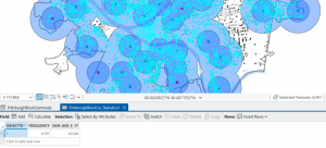
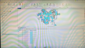
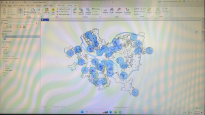
This was the final chapter of this week, and entered the third part of the book that focuses applying more advanced GIS technologies. Chapter nine’s focus was spatial analysis and shows us how to use buffers, multiple-ring buffers, create service areas of facilities, and preform cluster analysis. I focused on Tutorial 9-1 for this chapter. The focus of this tutorial was using buffers for proximity analysis. It starts by showing us how to use the Pairwise Buffer tool, which allows us to find what is in proximity to the feature being buffered. For this one, it has us create a buffer around the pools in Pittsburg. I had no trouble in the first step and was able to create the blue buffer pictured below. This was a really cool feature and made it really easy to visualize where all the pools are. It then had us use block centroids to sum the number of youths. This opened up the teal circles and the graph pictured below. I also had no trouble with this step. For the Your Turn portion of this tutorial, it asked to create a mile buffer around the pools. I attempted this by adding the same commands, but changing Distance to 1 U.S. Survey Mile. This created a new and larger buffer around the blue circles. However, the buffer looked much different from the picture and took up more space which makes me wonder what the correct measurements would be or if anything else needed changed. It moves on and shows us how to create multiple ring buffers using the same data. Overall, this chapter was relatively simple compared to the last chapter.

Chapter 7:

I found this chapter really fun, especially during the sections on creating, deleting and smoothing polygon features. I feel like this specific part of the textbook will be extremely helpful to me for the final portion of the course as I apply what I’ve learned in imaginary GIS applications. This chapter leaned more towards manipulating and creating your own data points and polygons rather than working on ones we’ve been given thus far. While being one of the shorter chapters, I feel like this is the one I will be applying the most.

 

---

Chapter 8:

Chapter 8 was also one of the shortest chapters we have had to do for the course, and it provided a lot of useful information about geocoding (a GIS process that matches location fields in tabular data to corresponding fields in existing feature classes) using zip codes. It also gave a step-by-step guide on how to geocode using street addresses using the sample data we were given. A key step in this process is knowing how to use the Geoprocessing tool on different data layers, which the textbook explained in great detail. I will be referring to this chapter a lot in the future, not just during the final but in my other courses that require a base level understanding of GIS.

 

---

Chapter 9:

I found this chapter extremely interesting, as it gave me a lot of the base level information I will need to complete the Final for this course. It explained how to create and use buffers for proximity analysis, as well as how to use multi-ring buffers. Buffers can be very useful to policy-makers when they want to visualize the number of people who could be affected by a specific policy, as well as estimating travel distance or time on a street network. Learning to use the Pairwise Buffer tool, the Multivariate Clustering tool and how to perform Network Analyses was very helpful to me, and I will be applying a lot of this knowledge in my Final.

Chapter 7

This was my favorite chapter!

I have to admit, the idea of creating features within the software was something I one hundred percent expected to be brought up way earlier. Although I do not understand its placement I found the activities in this chapter to be rather fun and rewarding. The whole thing was reminding me of a course I took in High School about using Autodesk Inventor and I was very easily able to apply what I have learned from then to this.

The different selections necessary to execute the activities were far less impressive. It seemed that after moving/adjusting the polygons, I had to click like three things in three different toolbars to get back to the standard “click and move” function. This was highly annoying, but not nearly as bad as the ways to edit the properties of the polygons themselves. I would have appreciated a much more simpler form of  changing the names of these campus buildings to something vaguely funny.

 

 

 

 

 

 

Chapter 8

Very short chapter with very little in my opinion to write home about. (Ironically, I am writing about it.)

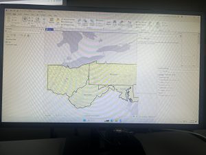
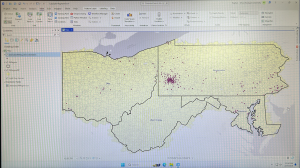
Chapter eight mainly had tutorials on how to mark different postal codes and street addresses within the map software using the examples of Ohio, Pennsylvania, West Virginia, and Maryland. Despite how short the chapter was, I found the methods used in the books to be rather finicky and many times it made references to toolbars or menus that I swear to god I have never heard of before and to which the search/help function on ARCGISPRO gave little help on.

Chapter 9

Final chapter!

I was very much so intimidated going into this chapter as the textbook labeled this as an “advanced application” or something like that but frankly, it was not all that bad. It was a pretty average chapter all things concerned. Chapter nine just discussed proximity analysis and how to use buffers and other maps to cross reference data with it. The example in particular used locations of town pools as well as locations of possible customers to the pools.