Don’t cry over GIS, it isn’t worth it. Thank you again.
Month: October 2022
Lee Leonard Week 4 and 5
I’m hoping no one sees this. I condensed week 4 and 5 into one PDF and intend to do the same for the data inventory and final. Thank you!
Final- Sturgill
Final-GEOG191 (1) . I hope this works and is accessible!
Final- Cailee Plunkett
I’m hoping this link works, but here is my final.
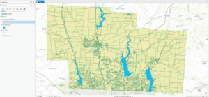
Delaware Data Inventory- Cailee Plunkett
Zip Code
> Contains all zip codes in Delaware County, Ohio
Recorded Document
> Contains points that represent recorded documents. These include subdivisions, vacations, surveys, etc.
School District
> Contains all school districts within the county
Map Sheet
> Contains all map sheets within the county
Farm Lot
> Identifies all farm lots and their boundaries in both the US Military and Virginia Military survey districts
Township
> Identifies the geographic boundaries of each township within the county
Street Centerline
> Shows the center of pavement on public and private roads within the county
Annexation
> Contains the annexations and conforming boundaries from 1853 to now
Condo
> Shows all condominium polygon boundaries within the county
Subdivision
> Shows all subdivisions and condo polygons within the county
Survey
> A shapefile of point coverage that shows land surveys within Delaware County
Dedicated ROW
> Consists of all designated Right-of-Way lines within the county, and is updated daily
Tax District
> Contains all tax districts within the county
GPS
> Shows all GPS identified monuments established between 1991 and 1997
Original Township
> Contains the original boundaries of the townships within the county before tax district changes affected their shapes
Imagery 2019
> Aerial imagery of Delaware County from 2019
Hydrology
Shows all major waterways within the county
Precinct
> Shows all voting precincts within the county
Parcel
> Consists of the polygons that represent parcel lines within the county
PLSS
> Consists of the Public Land Survey System polygons in both the US Military and Virginia Military Survey Districts of Delaware County
Address Point
> A spatially accurate representation of all certified addresses within Delaware County
2022 Leaf- On Imagery (SID File)
> 2022 imagery
Building Outline
> Contains building outlines of all structures within the county
Delaware County Contours
> Contains two-foot contours for the county
2021 Imagery (SID File)
> Imagery of the county for 2021
Delaware County E911 Data
Address mapping intended to aid with 911 response
Week 5- Plunkett
Chapter 6:
> Domains provide a way for you to constrain input information by limiting the choice of values for a particular field
> Using domains maintains data integrity- does not allow other values to be added during data collection
Chapter 7:
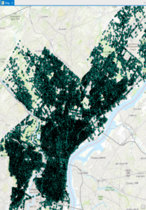
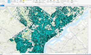
> The process of creating map features from addresses, place names, etc. is geocoding.
> To geocode addresses, you need an address table, reference data, and an address locator
Chapter 8:

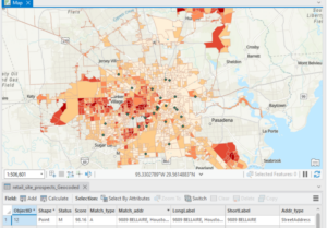
> In the first exercise, I created a kernel density to see where areas of high density may occur.
> Kernel density: the density calculated of point features around each output raster cell
> Temporal data represents a state in time
Chapter 9:
> Rasters are composed of a grid of cells instead of x, y coordinates
> Used to define and record geographic phenomena
> The reclassify tool is used to replace raster cell values with new cell values so that the rasters can be combined

Chapter 10:
> Dynamic labels are created when ArcGIS places labels for features in a layer with one click based on predetermined labeling rules.
> Useful for most mapping projects, but label positions can change depending on map scale
Week 4- Plunkett
Chapter 1:
> Point, line, and polygon data is also known as vector data
> Collecting measured values for any location on the Earth’s surface to form a digital surface is known as a raster.
Chapter 2:
> .aptx is the typical project template
>.aprx is a project file
>.ppkx is a project package
> The contents pane allows you to modify a map’s layers
> Learned how to select individual features
> Learned how to change feature symbols, display feature symbols, use the measure tool, and package my project to share online.
> Learned how to convert a 2D map to a 3D one
Chapter 3:
> An attribute query is a request for features in a table that meet user-defined criteria.
> Using an attribute join operation, we can join the spreadsheet table to the existing attribute table, as long as there is a common attribute field in each table
> Columns are often called fields.
> Fields include Object ID, which is a unique identifier assigned to every row in a table
> A layer file is a saved symbology scheme that points to a specific source datasheet
> A layer package bundles the layer file along with the source data
> Joining data based on location is a spatial join- this allows you to define a spatial relationship between two layers and combine their attributes in a new output layer

Chapter 4:
> A shapefile stores geometry and attribute data for one feature
> A geodatabase is a storage container where sets of features are stored into feature classes
> Nonspatial tables do not have well-defined geometry as feature classes do
Chapter 5:
> Python is a coding language that is compatible with ArcGIS
> You can define a workflow in the ‘tasks’ pane
Week 3- Plunkett
Chapter 5: Finding What’s Inside
> Finding what’s inside allows you to see whether an activity occurs inside an area or to summarize info. for several areas to compare
> You can draw an area boundary on top of features, use an area boundary to select the features inside and summarize them, or combine area boundaries and features to create summary data.
Selecting features inside the area:
> Good for getting a list or summary of features inside a single area
> Good for finding what’s within a certain distance of a feature
> You need the dataset containing the areas and a dataset with the features
Overlaying areas and features:
> Good for finding which features are in several areas or how much of something is in one or more areas
Using the results:
> Most common summaries include the count and frequency
Summary of a numeric attribute:
> Most common ones include the sum, average, median, and standard deviation
Overlaying areas with discrete features:
> The GIS tags each feature with a code for the area it falls within and assigns the area’s attributes to each feature
Vector method: GIS splits category or class boundaries where they cross areas and creates a new dataset with the areas that result. Each new area has the attributes of both input layers
Raster method: When you combine raster layers, the GIS compares each cell on the area layer to the corresponding cell on the layer containing the categories. It then counts the number of cells of each category in each area, calculates the areal extent by multiplying the number of cells by the area of a cell, and presents the results in a table.
Chapter 6: Finding What’s Nearby
> Finding what’s within a set distance identifies the area, and the features inside the area, affected by an activity.
Things to consider:
> Is what’s nearby defined by a set distance, or by travel to or from a feature?
> Are you measuring what’s nearby using distance or cost?
> Are you measuring distance over a flat plane or using the curvature of the earth?
Info. you need from the analysis:
> List: example is a parcel ID and address of each lot within 300 feet of a road repair project
> Count: can be a total or a count by category
> Summary statistic: can be a total amount, an amount by category, or a statistical summary (standard deviation, average, etc.)
Finding what’s nearby:
> Straight line distance: specify the source feature and the distance, and the GIS finds the area or the surrounding features within the distance
> Distance or cost over a network: specify the source locations and a distance or travel cost along each linear feature
> Cost over a surface: specify the location of the source features and a travel cost. The GIS creates a new layer showing the travel cost from each source feature
Creating a buffer:
> Specify the source feature and the buffer distance
> You can save the line as a permanent boundary or use it temporarily to find out what or how much of something is inside the area
> If you have several source features, GIS can buffer each source at the same distance or have it draw a variable distance buffer based on an attribute of each
> You can also specify several source features and the GIS will create buffers around all of them at once.
> If you want to find features within the distance of more than one source feature, you’ll need to create separate buffers and select the features surrounding each
Spider diagram: if a location is near two or more sources, GIS draws a line to each
Creating cell distance ranges: each cell potentially has a unique value. You display the the values using graduated colors so you can see the patterns
> You can summarize either discrete features or continuous data within the distance
> You can limit the area for which the GIS calculates distance by specifying a maximum distance
Chapter 7: Mapping Change
> Geographic features can change in location or change in character or magnitude
> Mapping change in location helps you see how features behave so you can predict where they might move
> Mapping change in character or magnitude shows how conditions in a given place have changed.
The geographic features:
> You can map discrete features that physically move, or events that represent geographic phenomena that change location
> Discrete features can be tracked as they move through space
> Might be individual features you can map paths for (hurricanes, vehicles, animals, etc).
> Events such as crime or earthquakes can represent geographic phenomena that occur at different locations
Measuring time:
> You can measure time in trends, ‘before and after,’ and through cycles
> If you’re mapping trends, you need to determine the interval, the number of dates, and the duration. The duration divided by the number of dates gives you the interval.
Mapping change:
> Time series: good for showing changes in boundaries, values for discrete areas, or surfaces.
– Good for showing the patterns of individual movement if you’re tracking many features, such as 911 calls over time.
> Showing fewer maps, farther apart in time, may make a change in values easier to see
> Showing more maps closer together in time may reveal patterns that are missed when using fewer maps
> It is difficult to compare more than five or six maps at a time
> Tracking map: good for showing movement in discrete locations, linear features, or area boundaries.
– Good for showing incremental movement of discrete features
> Linear features are often mapped before and after an event
> Measuring change: measure and map change to show the amount, percentage, or rate of change in a place.
Abbey S Final
Hopefully this shows up!