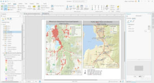
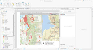
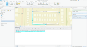
Hopefully this shows up!
Author: amsetlik
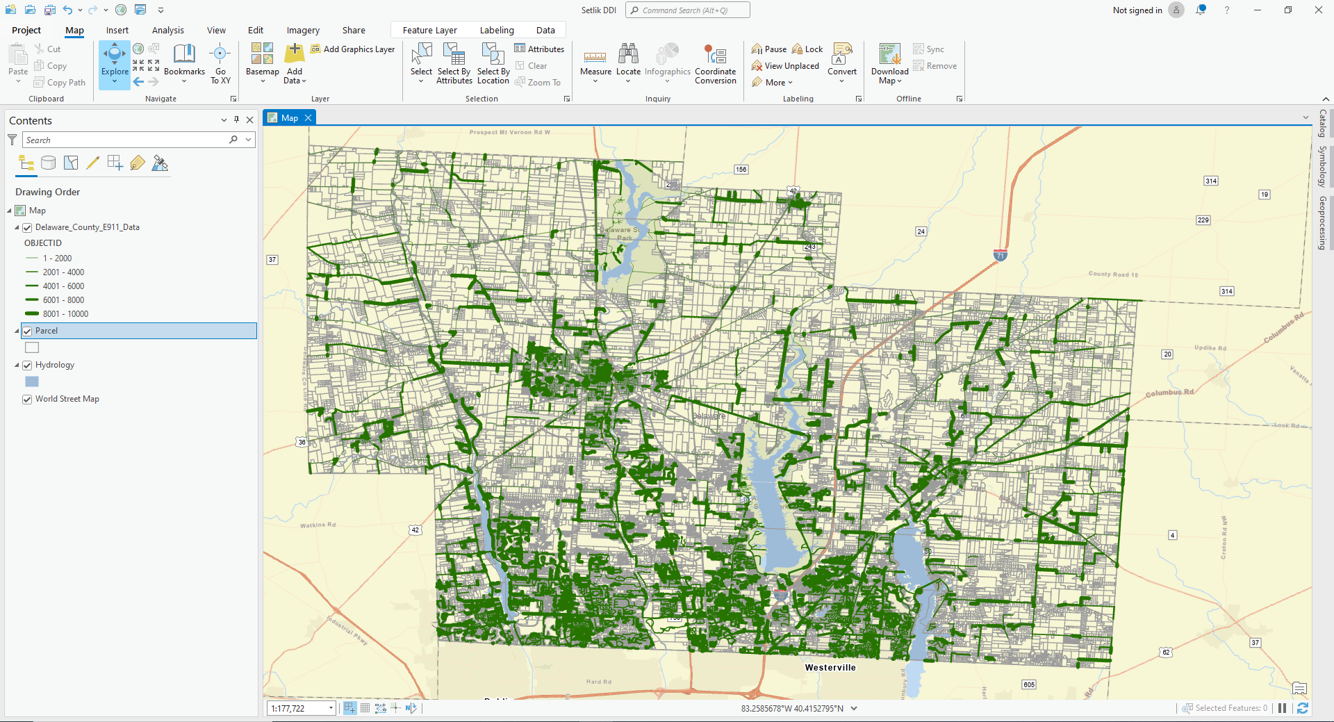
Abbey S Delaware Data Inventory
DATA SUMMARY
- Zip Code
- Contains all zip codes in Delaware County
- Recorded Document
- Points that represent recorded docs in Delaware County Recorder’s Plat Books (how purchased property is divided in an area), Cabinet slides, and Instruments
- School District
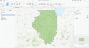
- Consists of all school districts in Delaware County
- Map Sheet
- Consists of all map sheets in Delaware County
- Farm Lot
- All farm lots in US Military and VA Military Survey of Delaware County
- Township
- Created to identify geographic boundaries of each township in Delaware County
- Street Centerline
- LBRS depict center of pavement of public/ private roads in Delaware County
- Annexation
- Contains annexation data and conforming boundaries
- Condo
- Consists of all condominium polygons in Delaware County
- Subdivision
- All subdivisions and condos in Delaware County Recorder’s office
- Survey
- Locations of the survey plat
- Dedicated ROW
- Shows all dedicated right of way polygons in Delaware County
- Tax District
- All tax districts in Delaware County
- GPS
- All GPS monuments est. 1991 and 1997
- Parcels-DXF
- All parcels in Delaware County
- Subdivsions-DXF
- All subdivisions and condos in Delaware County Recorder’s office
- DXF- kind of vector file (I think)
- Original Township
- Original boundaries of townships in Delaware County
- Imagery 2019
- Raster layer
- Hydrology
- All major waterways in Delaware County
- Precinct
- Polygons that determine voting precinct boundaries in Delaware County
- Parcel
- All parcels in Delaware County
- PLSS
- Contains polygons of boundaries of 2 land survey districts in Delaware County
- Address Points
- All addresses in Delaware County
- 2022 Leaf- on imagery (SID file)
- Image collection
- Building outline
- All building outlines for structures in Delaware County
- Delaware County Contours
- File geodatabase
- 2 foot contours for Delaware County
- Address Points- DXF
- CAD Drawing
- LBRS provides spatially accurate placement of addresses
- Street Centerlines- DXF
- CAD drawing
- Depict center of pavement of public and private roads in Delaware County
- Building Outlines- DXF
- CAD drawing
- 2021 Imagery (SID file)
- Image collection
- Delaware County E911 Data
- Feature Service
Some of these data were self-explanatory, and others required a little more reading.
Definitions:
- CAD drawing- Detailed illustration using vector/ raster based graphics to create traditional drafts
- Feature service- Serve feature data and nonspatial tables over internet
- File geodatabase- Collection of files that can store spatial and nonspatial data
Abbey S Week 5
Chapter 6:
6a
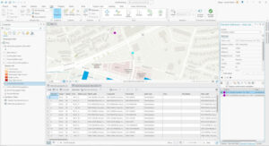
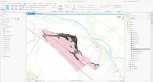
- I was able to work on the tree inventory data up until I had to publish it because I kept getting a pop up that my account does not have publishing privileges?? Idk if anyone else ran into this problem, but I was not able to find a solution so I couldn’t complete the rest of chapter 6 🙁
- Here’s my sad little screenshot
Chapter 7:
7a
- Geocoding- able to create data from collected points of interest
- To geocode addresses , you need-
- Address table (list of addresses stored as database or text file)
- Reference data (usually streets layer, where addresses are located)
- Address locator (contains reference data+ geocoding rules/settings)

7b
- Geocode location data
7c
- Buffers- polygons created around features at specified distances
- Using GIS in this way can help businesses evaluate the best locations

Chapter 8
8a
- Temporal data
- Data w time attribute
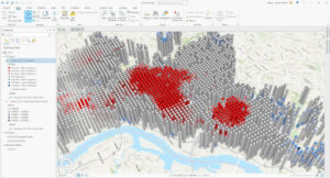
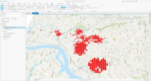
- Kernel density
- Calculates the density of features in an area around those features

8b
- I think the 3d stuff is pretty cool 😀
8c
- Not much to comment on this exercise, but the scene is much easier to look at now
8d
Chapter 9
9a
9b
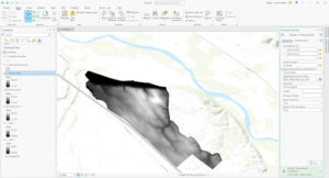
- At this time, no parts are in complete shadow
- 3 to 4 planting sites have low-slope topology
- 4 planting sites include land that faces S, SE, or SW
- No planting sites in shadow @ 2pm
- Some sites meet ⅔ criteria, but not all 3
9c
- Greenfield fine sandy loam, Xerorthents, loamy, Rincon clay loam
- Yes, some of the potential sites have been planted
Chapter 10
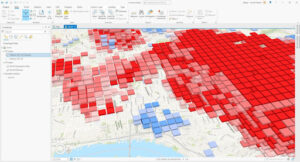
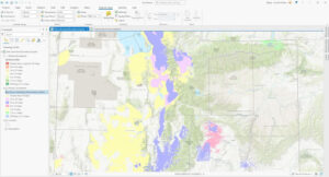
10a
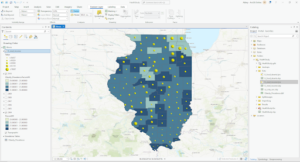
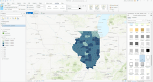
- 43 areas are fixed wireless technology
- For whatever reason I wasn’t allowed to change the color scheme
10b
- Labels- based on feature attributes and placed by/ on a feature
10c
- Map frames- containers for maps in a page layout
- Changing the map extent does not affect actual map
- Legend helps readers understand the features on the map
- Scale bar indicates the size of distances/ features on a map
- North arrow indicates north
10 d
Abbey S Week 4
Chapter 1:
- GIS is composed of 5 parts: hardware, software, data, procedures, and people
- Can be used to map relationships, patterns, and trends in addition to simple cartography
- Interesting how GIS has been around since the 60’s. I wonder how difficult it was to use it back then
- Point, line, polygon data = vector data
- Features of same type = layers
- Raster= digital surface
- Attributes= in depth data
- Don’t be like me and do the exercises in the classic map view, and then get confused as to why everything looks different


Chapter 2:
Exercise 2A
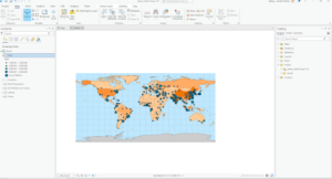
- PM concentrations are highest in Africa
- To restore contents, go the ‘View’ and select contents
- Geoprocessing toolbox is right next to contents
- Shanghai has the largest population
Exercise 2B
- Symbology= the way GIS features are displayed on a map
- The distance between San Antonio and Toronto is 1,440.32 mi

Exercise 2C
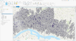
- The highest building is 339.8 ft
- Extrusion= stretching flat 2D features vertically to appear 3D
- This was cool- I felt like I was playing the Sims lol

Chapter 3
Exercise 3A
- The field name that indicates the state within the which the county features are located is called STATE_NAME
- 10575 residents of Wayne county are between 22-29 yrs
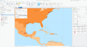
- Definition query: limit visible counties to only in Illinois, but source data will not change
- Clip: Select data based on layer of boundary (However, Illinois boundary not defined)
- Select and export: select counties in Illinois and export to new dataset
Exercise 3B
- Columns= fields
- There are six years of data represented
- Graduated colors= features are assigned a color that represents a quantity
- Classification methods:
- Manual interval classification
- Modify classification breaks manually with manual intervals
- Equal interval classification
- Range of data is equally divided by the number of classes chosen
- Defined Interval Classification
- Similar to equal interval, but define interval size to determine class number
- Quantile classification
- All classes have same number of features
- Natural breaks classification
- Based on natural groupings inherent in the data
- Geometric interval classification
- Creates class breaks that are based on class intervals with a geometric series
- Standard deviation classification
- Creates classes according to a number of standard deviation classifications
- Manual interval classification
- I did not see a clear correlation between income and 2010 obesity rates
Exercise 3C
- I was not able to retrieve the infographics even though I was signed in to ArcGIS online 🙁
Exercise 3 dimension
- There are 4 food deserts in Knox county
- Spatial join= define spatial relationship between 2 layers and combine attributes into an output layer
Chapter 4
Exercise 4A
- Coordinate systems
- Geographic coordinate system- uses latitude and longitude to define locations of points
- Projected coordinate system- uses map projections to transform longitude and latitude coordinates into planar coordinates
- On the fly projection
- Projected coordinates on first layer applied to subsequent layers
- Metadata
- Textual info about dataset
Exercise 4B
- Snapping= magnet
- The selected line has 4 vertices
Exercise 4C
- The shape area value was halved
Chapter 5
Exercise 5A
- Conflict types:
- Riots/protests
- Battle
- Remote violence
- Strategic development
- Violence against civilians
- 727015 fatalities
Exercise 5b
- 41 riots/protests
- 71 fatalities
Exercise 5c
- Layer by attribute and Summary statistics are combined
- 26323 fatalities
Abbey S- Week 3
Chapter 5: Finding What’s Inside
You can map what’s going on inside an area if you want to compare different areas or if you want to show what locations need action
- What’s inside a single area vs multiple areas
- Features either discrete or continuous
GIS can be used to:
- Figure out whether a feature is inside of an area
- Find all features in an area
- Find number of features in an area
Some features may be partially in an area
- Only use portion actually in the area
Three (3) ways to find what’s inside:
- Draw features/ areas
- Effective visual
- Need dataset of area boundaries and dataset with features
- Selecting features within an area
- You determine the area/ layer, and GIS selects all features
- Good summary of features in an area
- Cannot use for surfaces
- Overlaying areas and features
- Good for finding which features are in a number of areas
- Requires more processing
Based on the information provided in the book, it seems like the second method is not particularly effective. It cannot be used for surface features and overlaying features (method 3) allows you to see the same information.
More details on each method:
Drawing areas/ features
- Make sure it is easy to see what features are in the area
- Locations and lines require different symbols/ thicknesses in order to differentiate them from each other
- To map discrete areas:
- Lightly shade the area
- Make the area translucent or shade the area with a pattern
- Draw only the boundary of the area
- To map continuous data:
- Same as discrete
- Place a screen on the outside area to emphasize what’s in the area
Selecting features in an area
- You determine the features and area, and GIS will let you know what features are within the boundaries of an area
- GIS does not distinguish which areas the features are in (L)
- You can use this method to generate a report of the results, which can be used to relay information to the masses
Overlaying areas with continuous categories/ classes
- GIS uses vector/ raster method to overlay info
- Overlaying areas on areas requires slivers
- Slivers are small areas that are slightly offset
- An area with an areal extent less than the smallest dataset
- Raster vs vector
- Vector- more precise but more processing
- Raster- more efficient, prevents slivers, but sometimes less accurate
Chapter 6: Finding What’s Nearby
What’s occurring around a feature?
- Important for projects that need to be conscious of the surrounding area (development, demolition, etc.)
- Measure line distance, distance/ cost over a network, or cost over a surface
Taking the curvature of the earth into account
- Planar method is used for smaller areas such as cities, states, or countries
- Geodesic method good for regions and continents
- Will be displayed with the curvature of the globe
Information from analysis
- List
- Count
- By total
- By category
- Summary statistic
- Total amount
- Amount by category
- Statistical summary
- Average
- Minimum/ maximum
- Standard deviation
Number of ranges
- Inclusive rings- how total amount increases as distance decreases
- Distinct bands- compare distance to other characteristics
Straight line distance:
- Defines area of influence around an area
- Quick ‘n easy
- Only gives an approximation
- Create buffer to define a boundary
- Select features in order to find features in a given distance
- Calculate feature-feature distance to assign distance to locations
- Create distance surface to find continuous distance from source
Distance/ cost over a network:
- Measures travel over a fixed infrastructure
- More precise
- Needs an accurate network layer
- GIS identifies all lines in a network
- Source locations in networks are centers
- Street neworks
- Street segments (edges)
- Intersections (junctions)
- Tagged with cost to travel from center to surrounding locations (impedance value)
- Set travel parameters
- Can specify cost for turns from one segment to another
- More than one center
- GIS assigns segment to each concurrently
Cost over a surface:
- How much area is within an overland travel range
- Allows you to combine multiple layers
- Needs data preparation
- Creating a cost layer
- The book uses an example of the cost between deer traveling through open forest vs thick underbrush, and how it would be easier for deer to travel through open forest (yay animals). Therefore, open forest= lower cost
- Reclassify layer based on existing attribute
For me, this chapter really showed how specific you can get with GIS, especially when it came to determining traveling costs over a network or surface!
Chapter 7: Mapping Change
Mapping change allows us to make predictions on what the future could look like (big emphasis on meteorology)
Types of change:
- Location
- How features will move
- Can map features that physically move or geographic phenomena that change locations
- Discrete features can be tracked as they move through space (organisms or meteorological events)
- Events happen at different locations (earthquakes, deaths)
- Showing patterns of movement for individual features or
- Number of large yet distinct features
- Character/ magnitude
- How conditions in a given place have changed
- Discrete features are changes throughout a period of time
- Data summarized by area are presented as percentages or totals
- Continuous categories show the type of features in a place
- Continuous values are quantities that fluctuate
- Magnitude- similar issues as mapping most and least (ch. 3)
- Character- the way categories are defined may differ between dates
Measuring time:
- Three types of patterns
- Trend- change between two periods
- Increasing or decreasing?
- Before/ after- self explanatory
- Impact?
- Cycle- change during recurring time period
- Patterns?
- Trend- change between two periods
- Choosing time interval
- Need to choose interval if given a range
- Should be long enough to show change, but include all info
- Three ways to map change
- Time series- change in boundaries, discrete areas, surfaces
- Good visual impact, easy to understand
- Need comparisons
- Tracking map
- Showing movement of discrete locations, linear features, area boundaries
- Easier to see subtle movement compared to time series
- The more features, the harder to read
- Measuring change
- Show amount, percentage, rate of change
- Shows difference in values
- Omits actual conditions
- Time series- change in boundaries, discrete areas, surfaces
Number of maps to show
- Fewer maps spaced longer apart shows more drastic change
- More maps account for possible patterns that may have been missed
- More maps are more overwhelming for the viewer
Results
- Showing tables and graphs can supplement what you are trying to show thru maps
Mapping linear features
- Differentiate between each point with labels, colors, or symbols
Mapping contiguous features
- Draw boundaries for areas at each date/ time
Mapping events
- Use different colors for each time period
Abbey S- Week 2
Chapter 1: Introducing GIS Analysis
Map uses:
- Where things are
- Most and least
- Density
- What’s inside
- What’s nearby
- Change
GIS can be simple, like a basic map, or a more complex figure with multiple layers (like an onion)
Geographic features can be discrete, continuous phenomena, or summarized by area
- It’s important to understand what you’re mapping!
- Discrete features can be pinpointed
- Businesses represented by number of employees
- Continuous phenomena are always present, and we map the changes (e.g. temperature)
- Interpolation– values that are assigned to areas in between points
- Non continuous data can be continuous if showing variation across a given location
- Centroid– center points
- Summarized data is used for density/ counts of individual points in a certain area
- Would this mean the individual points would be discrete features, and the presence of a boundary is what makes it summarized data?
Geographic features can be represented using vector or raster
- Vector-
- Feature is a row on the table
- Shapes are defined by x and y
- Lines= coordinate pairs
- Shapes= closed polygons
- Raster-
- Features are a matrix of cells in continuous space
- 1 layer= 1 attribute
- Sizing is important! Too large and info will be lost, too small and it takes longer to process
Geographic attributes:
- Categories
- Groups of similar things
- Represented by numeric codes or text abbreviations
- Ranks
- Order from highest to lowest
- Used to compare features that are harder to quantify
- Counts
- Number of features on a map
- Amounts
- Measurable quantity associated with a feature
- So a count would be the number of circles on a map, and an amount would be the number that each circle represents?
- Ratios
- Shows relationship between two quantities
- Dividing one quantity by another
- Proportions- part of a total value
- Density- distribution of feature per unit area
Chapter 2: Mapping Where Things Are
Maps show where action is needed. It is important to know what features need to be present and how to display them.
Creating a map:
- It needs to be relevant for your audience
- Avoid unnecessary details
- Smaller maps need to be concise and only show important aspects, while larger maps are able to provide more detail
- Features need to be geographically assigned!
- Categories help identify groups of features
- Types and subtypes
- If only one type, all features should be the same shape
- Subsets used for individual locations
- Context is important!
Categories can reveal patterns
- Can provide an understanding of how a place functions
- Most people can distinguish up to seven colors/ patterns on a map
- I thought this was really interesting! Because of this, it is strongly encouraged that there are no more than seven categories displayed at once
- The spacing of the categories also plays a role
- I assumed that categories would be more easily distinguishable if they were spread out, but Mitchell says the opposite.
- You may have to lose some information in the process of making it easy to read
- How would you determine what information is needed the least? How often does this happen?
Grouping categories can change the viewer’s perception of the information
- Assign detailed and general category codes
- Create a table with detailed and general category codes side by side
- Assign the detailed categories a symbol that represents the general category
Symbols
- Size needs to be “just right”- large enough to be distinguishable, small enough as to not obscure
- Use different widths to distinguish lines
- Patterns as well ( dashed lines, dotted lines, etc.)
Geographic Patterns
- Clustered distribution- Features more likely to be found near other features
- Uniform distribution- Features less likely to be found near other features
- Random distribution- Features likely to be found at any given location
Chapter 3: Mapping the Most and Least
Add a layer of information that can be useful instead of just a location on a map (What is the elephant population at this point, and why is it higher than the population at a different point?)
Can map all 3 types of quantities (discrete features, continuous phenomena, summarized area)
Continuous phenomena can be portrayed as a gradient of colors-
- More saturated= most
- Least saturated= least
- Red= =high
- Blue= low
- etc
As I am going through the chapters, I noticed that Mitchell will repeat the same definitions for words previously mentioned. Some people may find that annoying but I appreciate the repetitiveness as it helps me remember what certain words mean.
Creating Classes
Simplicity is key when it comes to comparing values
- Balance between portraying accurate data values and generalizing data enough to show a pattern
- Map example:
- Shading each area with a unique shade based on its data value can muddle the image (too many colors!)
- It is much easier to create classes that each contain a range of the values (less color good)
Mapping individual values can be overwhelming for viewers. The data may be more accurate but not necessarily better.
Standard Classification Pyramid Schemes
- Natural Breaks
- Based on natural groupings of values
- Use if data is unevenly distributed
- Quantile
- Each class has same number of features
- Use if data is evenly distributed and you want to show relative difference between features
- Equal Interval
- Difference between high and low values is same for every class
- Use if data is evenly distributed and you want to highlight the difference between features
- Standard Deviation
- Placed based on how far they deviate from the mean
- Use if data is evenly distributed and you want to highlight the difference between features
How does one decide between equal interval and standard deviation?
Map type is dependent on type of features-
- Discrete locations/ lines
- Graduated symbols
- Charts
- 3D view
- Discrete areas
- Graduated colors
- Charts
- 3D view
- Spatially continuous phenomena
- Graduated colors
- Contours
- 3D view
In conclusion, you can’t go wrong with a 3D view
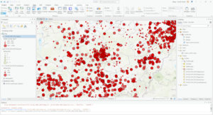
Chapter 4: Mapping Density
Shows you where the highest concentration of features are
More useful for mapping patterns
Looking at the images I can already tell that it is much easier to comprehend a gradient of density instead of a bunch of lines or dots
Two ways to map density-
- Density map
- Dot maps
- Calculate density value to create a shaded map
- Density surface
- Raster layer
- Requires more effort
- Trade offs
- Use density map if you have data summarized by area, but beware if you want exact centers of density
- Use density surface if you have individual features and are prepared for more data processing
When creating a shaded map, make sure to limit the amount of colors/ shades used
Dot maps
- Allows for more detail
- Dots represent values in each area
- Dots that are larger represent more values, and will therefore be more spread out
- Make sure the boundary is larger than the dotted area
Density Surface
- This is where I start to get lost
- Cell size determines coarseness of the pattern
- Smoother= more data processing
- To calculate cell size:
- Convert density units to cell units
- Divide by the number of cells
- Take the square root to get one side of the cell
- When the cell size is too big, it starts to resemble a shaded map
- Usually shades of a single color are used
- Exception is standard deviation, where one color equals above mean, and another color equals below mean
- Contour lines connects points
- Lines closer together= rapid change
- Lines farther apart= slower change
Abbey S- Week 1
Hello! My name is Abbey Setlik and I’m a senior Zoology Major. I’m originally from Herndon, Virginia. I’m taking this class to better understand how GIS works since it seems to be a valuable tool for future jobs. This summer I worked in Dr. Wolverton’s lab and helped move my siblings into college. They are quadruplets so it was pretty busy. I am interested in field biology and wildlife rehabilitation.

I liked how the reading focused on how GIS is used in many different practices. As someone who is not very familiar with GIS, I was confused about the difference between spatial and geographical analysis. The author also explained how there were two ways to approach GIS: “where” spatial entities are and “how” we encode spatial entities. I believe, as someone interested in scientific research, that the question of “how” is more relevant to my field, but I can see how both might be applicable. I personally think that GIScience is more interesting that GISystems. From my understanding, GIScience interprets and questions the data generated by GISystems?
I found a study that looked at the earthworm population in northwestern Caucasus using GIS. The study wanted to see whether the two species of earthworm preferred different forest locations, whether they were confined to different areas in any way and the general distribution of the two species across the study area. GIS came in handy especially when it came to answering the last question. The results of this study found that both species of earthworm inhabited all of the different types of forests, with the population the most abundant in coniferous-deciduous forests, and the least abundant in pine forests.
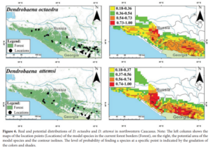
GIS was used to visualize the distribution of both species of earthworm.
GERASKINA, ANNA and SHEVCHENKO, NICOLAI (2019) “Spatial distribution of the epigeic species of earthworms Dendrobaena octaedra and D. attemsi (Oligochaeta: Lumbricidae) in the forest belt of the northwestern Caucasus,” Turkish Journal of Zoology: Vol. 43: No. 5, Article 7. https://doi.org/10.3906/zoo-1902-31
I also found records that utilized GIS to look at wildlife-highway relationships. I remember reading that cicada numbers have drastically decreased due to pavement blocking their way to surface ground, so I found it cool that GIS was mentioned to analyze similar phenomena. The program aimed to reduce animal collisions and work with the land when creating roads. GIS was used specifically to pinpoint critical areas that needed to be changed in order to reach the goal of conservation. (Smith, Harris, Mazzotti, 1999)