Month: February 2024

Dataset:

Address point: This shows all of the confirmed and office addresses inside of Delaware County. This also is a spatially accurate display.
Annexation: This shows Delaware County’s annexations with their boundaries. This is updated as-need and has data from 1853 to present.
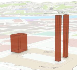
Building Outline 2021: This is a map from 2021 that shows all of the building outlines in Delaware County.
Condo: This shows all of the condominium polygons that are within Delaware County. However, it only shows the ones that have been recorded with the Delaware County Recorders Office.
Dedicated ROW: This shows all of the Right-Of-Way line data within Delaware County. This data is updated as-need and is created by updating daily.
Delaware County Contours: This shows the contour lines of Delaware County from 2018. These are given in two foot contours.
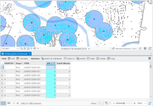
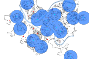
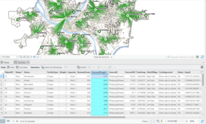
Delaware County E911 Data: This shows which address points from Address_Points layer that gives 911 agencies the information to determine the closest address to a caller.
Farm Lot: This data set shows determined farmlots. It includes those that are US Military and Virginia Military Survey Distinctions within Delaware County.
GPS: This includes all of the GPS monuments in Delaware County that were established in 1991 and 1997.
Hydrology: This shows all of the major waterways inside of Delaware County. This was created in 2018 using LiDAR technology and is updated as-needed.
MSAG: Short for Master Street Address Guide. This shows 28 political jurisdictions that create Delaware County.
Map Sheet: This shows all of the map sheets inside of Delaware County.
Municipality: This shows all of the municipalities that are inside of Delaware County.
Original Township: This shows what boundaries Delaware County originally had before tax district changes.
PLSS: Short for Public Land Survey System. This shows the Public Land Survey System polygons in US Military and Virginia Military Survey inside of Delaware County.
Parcel: This shows all of the cadastral parcel lines inside of Delaware County. These are represented as polygons.
Precinct: This shows the different Voting Precincts inside of Delaware County. This dataset is updated as-need.
Recorded Document: This shows points that are representative of record documents in Delaware County Recorder’s Plat Books, Cabinet/Slide and Instrument Records.
School District:This shows polygons for all of the school districts of Delaware County.
Street Centerline: This shows public and private roads inside of Delaware County. It represents the center of the pavement.
Subdivision: This shows all of the recorded subdivisions and condos in Delaware County Recorder’s office. This is updated on a daily basis.
Survey: This is a shapefile that shows surveys of land in Delaware County.
Tax district: This shows all of the different tax districts inside of Delaware County represented by polygons. The data is updated as-need.
Township: This shows the 19 different townships that Delaware County consists of. This is updated as-need.
Zipcode: This shows the zip codes of Delaware County represented by polygons.

Chapter 9:

• Tutorial 9-1: Learned how to use buffers for proximity analysis, run the pairwise buffer tool, select block centroids within buffers, and sum the number of a population
• Tutorial 9-2: Learned how to create and use multiple-ring buffers and use spatial overlay to get statistics by buffer area
• Tutorial 9-3: learned how to create multiple-ring service areas for calibrating a gravity model, create multiple-ring service area polygons, spatially join areas and pool tags, calculate pool use statistics for service areas, make a scatterplot, and fit a curve to the gravity model data points
• Tutorial 9-4: learned how to use network analyst to locate facilities and analyze optimal solutions
• Tutorial 9-5: Learned how to perform data cluster analysis and interpret the clusters

Chapter 10:

• • Tutorial 10-1: learned how to process raster datasets, examine raster dataset properties, import a raster dataset into a file geodatabase, set the geoprocessing environment for raster analysis, extract land use using a mask, symbolize a raster dataset using a layer file, create and symbolize hillshade for elevation, use hillshade for shaded relief of land use, and create elevation contours
  • Tutorial 10-2: learned how to make a density heat map, study the project location, run KDS, create a threshold contour layer for locating a service, use threshold areas to estimate data rates
  • Tutorial 10-3: learned how to build a risk index model explore the project area, standardize an input attribute, set the geoprocessing environment for raster analysis, create a new toolbox and model, add processes to the model, configure a kernel density process, configure the raster calculator process, run a model in edit mode, symbolize a KDS raster layer, and save its layer file, add variables to the model, use in-line variable substitution, use layer file to automatically symbolize the raster layer when created, and run a model tool

• Notes: for some reason when I ran my model it didn’t look like the pictures in the book

Chapter 11

• • Tutorial 11-1: Learned how to explore a global scene and its properties, navigate a scene with a mouse and keyboard keys, change the basemap, and exaggerate and apply a shade and time to a surface
  • Tutorial 11-2: learned how to create a local scene and TIN surface, set a local scene, create a TIN surface, change the scene’s surface and coordinate system, change the symbology of a tin
  • Tutorial 11-3: learned how to create z-enabled feature classes, digitize data and objects on surfaces using z-mode, display data and objects realistically
  • Tutorial 11-4: learned how to create features and line-of-sight analysis using lidar data, create a LAS dataset, generate a raster DSM and DTM, create an nDSM raster, create random points for buildings, add surface information to random points, assign maximum value (height) to random points, join  maximum z-value (height) to building footprints and display as 3D buildings, use lidar to determine bridge elevation heights, draw a bridge using Z Mode elevation, conduct a line-of-sight analysis

• Notes: something went wrong with running the different tools because my 3D Bldgs layer did not produce a lot of tall buildings. When I was entering in the information in the varying tools it was taking a long time to process on ArcGIS Pro, so I think that might have been where the issue was. The bridge section seemed to give me a lot of issues that I couldn’t figure out. For some reason, I did not have the layers that the 11-6 tutorial was asking me to turn on for the Smithfield Street section so I did not get to complete that section.

• Tutorial 11-5: learned how to work with 3D features, extrude floors, use a range slider to view building floors edit a building’s height using dynamic constraints and the attribute table 

• Tutorial 11-6: learned how to use procedural rules and multipatch models, apply building rules using stacked blocks, apply an international building rule, view multipatch models of buildings and street furniture
• Tutorial 11-7:learned how to create animation, add an animation to the project and create keyframes, play an animation and change the duration, create a pause, add and delete keyframes, create a movie from the animation

Screenshots:

Chapter 9: Spatial Analysis: Buffers, service areas, facility location models, and clustering

9.1

• A buffer is a polygon surrounding map features of a feature class. The radius of the buffer is specified and, generally, the radius is used to find what’s hear the feature being buffered
• Use the Pairwise Buffer Tool. Created buffer data can be summarized and analyzed using the Summarize tool

9.2

• Multiple ring buffers can be configured to be separate polygons to therefore allow you to select other features within given distance ranges from the buffered feature. Use the Multiple Ring Buffer Tool
• Use the Spatial Join Tool to use spatial overlay to get statistics by buffer area. It joins all attributes of the multiple ring buffer to block centroids and sums the numbers inside each ring

9.3

• Service areas are like buffers but are based on travel over a network, usually a street network dataset
• Gravity model: Assumes that the farther apart two features are, the less attraction between them. The falloff in attraction with distance is often nonlinear and rapid, as in Newton’s gravity model for physical objects, where the denominator of attraction is distance squared
• Use the 7 step workflow

9.4

• When using the location allocation model, demand is represented by polygon centroids, blocks, block groups, tracts, zip codes, and so on, for which you have data on the target population
• This section ran a model to choose the best of the locations to remain open using geographic access as the criteria. Use the Location Allocation tool under the Analysis tab, in the Workflows section, under Network Analysis to create a new layer in the Contents pane

9.5

• The goal of data mining is exploration. Data clustering, a branch of data mining finds clusters of data points that are close to each other but distant from points of other clusters
• A limitation of clustering is that there is no way of knowing true clusters in real data to compare with what an algorithm determines are clusters. Therefore, it is purely exploratory. 
• K-means clustering is a simple method in the Multivariate Clustering Tool that partitions a dataset with n observations and p variables into k<n clusters. K-means assumes that all attributes are equally important for clustering because it uses distance between numeric points as its basis. 5 clusters is generally most informative. 
• Each observation is a 3D vector and is characterized by its centroid with the corresponding means of each cluster variable

Chapter 10 Raster GIS

10.1

• Raster layers are for continuous features like satellite images, topography, and precipitation. You can also use raster layers to display an attribute such as population for large numbers of vector features like city blocks or countries. 
• Raster dataset is a generic name for a cell based map layer stored on a disk in a raster data format
• All raster datasets have at least one band of values. A band is comparable to an attribute for vector layers and stores the values in a single attribute in an array. The values can be + or – integers or floating point numbers
• Color capture and representation in raster datasets is important. Spatial resolution is the length of one side of a square pixel 
• The Raster to Other Tool can import a raster dataset into a file geodatabase 

10.2

• Kernel Density Smoothing (KDS) is a widely used method in statistics for smoothing data spatially. The input is a vector point layer, often of center points of polygons for population data or point locations
• It accomplishes smoothing by placing a kernel, a bell shaped surface with surface area 1, over each point. If there is population, N, at a point, the kernel is multiplied by N so that its total area is N. Then all kernels are summed to produced a smoothed surface, a raster dataset 
• The key parameter of KDS is its search radius, which corresponds to the radius of the kernel’s footprint. If the search radius is small, you will get highly peaked mountains, or, if large, you get wider rolling hills. 
• There are no exact guidelines on how to choose a search radius
• Can be good for representing demand surface for a good or service because its data smoothing represents the uncertainty of locations for future demand relative to historical demand
• Use the Kernel Density Tool

10.3

• Instead of code scripting, you can drag tools to a canvas and connect them in a workflow using ModelBuilder that you can use to run code. 
• If you have a reasonable theory that several variables are predictive of a dependent variable of interest such as poverty (whether the dependent variable is observable), the Dawes method contends that you can proceed by removing scale from each input arable and averaging the scales inputted to create a predictive index. This can be used for a risk index model. 
• Alternatively, you can assign different weights to different variables according to your preference. A good way to remove scale from a variable is to calculate z scores, subtracting the mean and dividing by the standard deviation for each value of a variable. Each standardized variable has a mean of zero and a SD of one (and therefore no scale).

Chapter 11: 3D GIS

11.1

• Global viewing model: For large extent, real world content in which the curvature of the earth is important
• Local viewing model: Small extent content in a projected coordinate system or for situations in which the curvature of the earth isn’t important
• Understanding a scene’s elevation surface, map units, and heights is important to the scene
• Use mouse wheel to tilt view, J or U on keyboard to move map up/down, A or D to rotate view clockwise or counterclockwise, W or S to tilt camera up/down, arrow keys to move the view, B and left arrow to look around, N to view true north, P to look straight down
• You can exaggerate a landscape with visual effects to help it stand out. It doesn’t change the elevation, just makes it more prominent. This can include lighting or time of day. Use the Elevation Surface Layer tab for light position and vertical exaggeration. Use Contents pane + properties of 3D scene for Date/time/illumination

11.2

• An advantage of local scenes is using your own elevation surface data such as triangulated irregular networks (TIN’s) or lidar data, using a projected coordinate system, managing features below a surface, and more accessible editing of data
• TIN’s are typically used for high precision  modeling of small areas to allow for the calculation of surface area and volume. They are also useful for viewing underground features. Use the Create Tin Tool 

11.3

• You can import 3D models and symbolize 2D features as 3D features and specify the source of your z-values when you create features
• The Current Z Control Tool is used to set the 3D elevation source for drawing or obtaining Z-values
• This is useful if more than one source is defined for a global or local scale, or if you java another source not already included in the map
• The Create Feature Class geoprocessing tool allows you to determine the required output feature class’ z-values
• I planted trees 🙂

11.4

• The generation of 3D buildings from lidar LAS datasets requires two surface models: a digital surface model (DSM) and a digital terrain model (DTM)
• A LAS dataset created from original LAS data provides fast access to lidar data without the need for data conversion to work with LAS files for a specific study area
• Use Create LAS Dataset tool
• DSMs represent the surface of the earth, including buildings, tree canopies, and other things that create a surface above the terrain. 
• LAS Dataset to Raster tool to create DSM
• DTM contains only the topology, a bare earth terrain surface. In many cases, it is the same as a digital elevation model (DEM). Before creating the raster, you filter the ground features
• An nDSM surface is the difference between the DSM and DTM surfaces that is normalized to the bare earth surface. You can use this raster surface to apply point features used for buildings to determine their height. Use the Create Random Points Tool. Assign z-values (height) from the nDSM raster surface using the Add Surface Information Tool. The Summary Statistics tool calculates the maximum Z Value for all buildings using the building’s random points

11.5

• Editing building polygons that are already 3D features to create multiple floors in a building and view floors using a range slider and manually edit polygons’ heights using z constraints
• Use the Duplicate Vertical Tool to create floors. You can also use this tool to copy points or lines (like furniture or pipes) in a positive or negative direction
• Add a range slider to visualize certain floors

11.6

• A CityEngine rule package (.rpk) is a file that contains a compiled rule and all the assets (textures and 3D models) that rule logic uses for creating 3D content. You can use these packages to create symbology that constructs and draws the procedural feature on the fly from the source data
• Another method that creates 3D models and stores them as a feature class is called a multipatch, whose features are a collection of patches that represent the boundary of a 3D object. It stores color, texture, transparency, and geometric data in its features
• When you apply procedural rules, you must display features as layers in a scene. The feature class polygon itself does not have to include Z Values, but it must be in a scene, and you can use 2D layers such as building polygons 

11.7

• Animations are created by capturing an ordered set of viewpoints (such as bookmarks) as keyframes and managing how the camera transition between them
• Find the animation tool under the View tab in the Animation group, then click Add
• To export an animation, in the export group, click the Movie button. In the export movie pane, in the movie export presets group, click Draft.

Chapter 9: 

This chapter introduced the Service Area Layer tool, which allowed you to add a network of things together. Overall, I didn’t have too much trouble with this chapter. I had some trouble with 9.3 because I could not add the new fields to create the scatterplot. I’m not really sure if it was an issue on my end or a bug in the tutorial. I also selected sum for the DemandWeight in 9.4 but I didn’t notice anything happening or change. I’m not sure if J was supposed to see a change or not. One thing new this chapter mentions is K-means which is used for clustering. I noticed under the clustering method that there were also k medoids. I’m curious what they could be for.

 

Chapter 10

This chapter introduced some new concepts and tools. One was the Kernel Density Smoothing tool which allowed you to smooth data spatially. We also got a chance to use ModelBuilder and build models in ArcGIS Pro. I think this tool could be really helpful if you are creating something for an employer. Additionally, the drop shadow under the process and output boxes symbolizing they have been run is neat. The Validate button can also be used  to ensure they are ready to run again or edit. I ran into a few issues with FHHChld weight and NoHighSchoolWeight. I learned that you have to click save before rerunning the model for there to not be error marks by these parameters. I eventually  got model to work

Chapter 11

I really enjoyed learning the keyboard shortcuts for moving around the map in this chapter. You can use J for down and U for up, A to go left and D to rotate right ,W and S tilt up and down , and B+move mouse allows you to look around in one spot sort of like a 360 tour video. By selecting Map properties for 3D-> illumination-> date and time, you can see the shadows and 3D features of the map in real time, which I thought was cool. I thought it was cool how we were able to display 3D images on the map like the trees. We also used the Create LAS Dataset tool in 11-4 which made a really cool 3D model of the city. I thought it was cool how we could modify the scale of the building in section 5. This was done by selecting Modify under the edit tab and the clicking scale on the pane that popped up. This would be really helpful if you were trying to design a new building.

My most favorite lesson from this book was section 7 where it goes over how to make a animation with the bookmarks. I thought that this was both really cool and something I could definitely see myself using in the future for an employer project. We were able to make the animation by going to manage bookmarks, then clicking the add button under animations on the view tab. Next, we clicked create first keyframe and then clicked the first bookmark. After selecting the second bookmark we clicked Append Next Keyframe at the bottom to add it to the animation. After repeating this with all the bookmarks, they were strung together into a short clip. You can also make it pause on a scene by clicking the scene and selecting hold. Click insert after moving to a different location on the map to make the animation go to that area.

Chapter 9
9.1- I got a bit confused during the Your Turn part and accidentally overridden the previous buffer, but I was able to fit it.
9.2- This made the last chapter’s “Your turn” seem like a redundant step, as it just taught us how to make multiple buffers.
9.3- The spatial joins failed. I am unsure as to what caused this error as I triple-checked the textbook instructions.
9.4- This one was a bit confusing, not in the steps, but more what I was trying to achieve.
9.5- While I was able to complete the tutorial, I believe I did the “Your Turn” part incorrectly, as my table did not match the book’s. However, I am unsure as to what the mistake was, as I tried to follow the instructions closely.

 

Chapter 10
10.1- For some reason, LandUse.Phg did not appear in my folder, although I completed all prior steps correctly. I am unsure if this was a personal or computer error.
10.2- Pretty straightforward and easy to follow. However, I wish the book would specify which tool it wants me to use, as there are sometimes different types with the same name.
10.3- The beginning “Your Turn” part confused me, as I felt I wasn’t given enough information to properly build the tool. I’m not sure if this affected the rest of the tutorial, as no helpful pictures of the map were included

Chapter 11
11.1- It was really cool to see the 3D version of the map, and the tutorial was very easy to follow
11.2- This was pretty straightforward
11.3- It was really cool seeing how to add trees to the map
11.4- I noticed that the processing tools in this chapter were really glitchy. They kept overriding my inputs, and I had to repeatedly redo the specific tools. I also received a lot of warnings, and at one point, the tool did not have settings that matched the textbook.
11.5- This one was pretty straightforward, although some of the instructions weren’t very clear.
11.6- The 3D street view did not load after 10 minutes so I decided to move on.
11.7- The animation was pretty intimidating at first, but it turned out to be really easy and super cool to see.

Chapter 9

9.1    I was ready to get started on a clean slate for part 3 so I’m glad this section was straightforward and simple. It was cool that when the buffers overlapped they just joined together. 

9.2    Creating multiple ring buffers was cool and I could see myself using it in a project in the future. Using the spatial join tool to see how many youths had good vs. excellent access was also very cool. Doing it with 3 rings was cool too.     

9.3     This section was a bit more tedious but it was good. It was cool to create the scatterplot.

9.4    I had no problems with this section. The lines looked really cool. It is interesting how many ways you can interpret one data set.

 

9.5    I liked doing the “Your Turn” part of this tutorial. I wasn’t sure if I knew how to do it but I figured it out as I went on.

  

Chapter 10

10.1     Changing the transparency of the land use map so that we could see the hillshade with it at the same time was so cool and I definitely see myself using this in the future.

10.2      This section was super easy. There was one part where I got confused: the book said to “run the tool” after symbolizing a layer. That was weird but I just ignored it.

10.3     I had quite a few issues with this section. When I was using the raster calculator, and I clicked on the raster names to add them to the calculation, they wouldn’t fill in so I had to write everything out. I also messed it up the first time so I had to do this a lot and it was very tedious. I also suspect something else went wrong because my poverty image did not look the same as the books. 

Chapter 11

11.1     This part was so cool!!! I feel like it might take a minute to get used to navigating with the keyboard but I feel like I’m already getting it! So fun! Picture from Denver.

11.2    This was another good section. I liked that we took out everything but the AOI. It would get kind of overwhelming with the whole world map. 

11.3   This section was so fun! The trees are so cute.

11.4    I didn’t really have any issues with this section, I’m just not sure I fully understand it. I know that a lot of the work done was to create the building heights, but I didn’t fully understand the process to get there. Creating the line of sight was so cool.

11.5   This tutorial was cool. Extruding the buildings was very simple.

.     

 

11.6    This section felt like google maps because of all the buildings on smithfield street.

11.7     Creating the video was so cool… I didn’t even know you could do that on ArcGISPro.

Chapter 9

• 9.1: Very short and straightforward, just learning to use the cluster tool
• 9.2: Again very straightforward, didn’t have any issue with the spatial overlay.
• 9.3: This one definitely took a while, at least longer than the others and was definitely more complicated. Did not have any technical issues that other classmates seemed to have experienced though.
• 9.4: At the very end of analyzing for the optimal situation, using the summarize tool didn’t seem to work. Or at least, no change occurred that I noticed.
• 9.5: Another straightforward section that just focused on changing symbols and labels.

Chapter 10

• 10.1: Very interesting to see the 3D landscape overlaid on the 2D map beneath.
• 10.2: Heat maps are among my favorite types of map… that sounds weird to say now that I think about it, but there is something about them that is inherently interesting so it’s fun to play around with.
• 10.3: Was ultimately very disappointed in the end result with this part. Took me two hours to find and put everything together from the model to the codes, and on the last step to run the tool I was met with some unknown error so it felt like a waste of time.

Chapter 11

• 11.1: Basically Google Earth but playing with exaggerated features and time based lighting.
• 11.2: I mean I suppose it’s interesting to see the different layers in different colors contrasting. All came together at the end seeing the landscape reflected accurately.
• 11.3: Shows how to add realistic objects to a map using z features and points.
• 11.4: The drawing of the bridge arch using z points didn’t work, and neither did the line of sight analysis
• 11.5: Very straightforward. Interesting to play around with the height of objects.
• 11.6: Was initially concerned since nothing was happening, then the building finally showed after playing with the properties in a different step. Interesting to see a realistic-ish building model.
• 11.7: I don’t think animation has ever been easier… I joke but its still cool to see an animation which is something like a 3D tour

Chapter 9- This chapter went fairly quickly and I did not run into any problems during these tutorials. Overall, this chapter went more in-depth on using buffers to analyze proximity and to find what’s near something. I don’t think we’ve had to use the buffers yet (unless I’m forgetting an earlier tutorial), but I really enjoyed learning how to use them and discovering more about how to analyze what is around certain places and how you can utilize ArcGIS tools to find useful things about the data. Looking ahead to the final exam, I think this chapter will come in handy, as using buffers is one of the options for the final. In the first few tutorials, I learned how to use buffers to calculate the total number of kids near public swimming pools. I think this would be a very useful tool for businesses to ensure that they are in the optimal location for their target demographics. You can also use the buffers to set location parameters as being excellent, good, or poor in proximity to a certain location- which could influence certain policies and encourage new builds. This chapter also went over some more Python concepts, how to create scatterplots to discover linear relationships, and how to use the Multivariate Clustering tool to analyze and interpret cluster data. The chapter used those last few concepts with regard to serious crimes, but I think that this kind of analysis could be used for various other reasons. 

MapCh9Crimes

MapCh9

MapBuffers2(Ch9)

Chapter 10- This chapter was all about rasters, and it was fairly short and straightforward. This was the first time we’ve had to really use a raster dataset, so we started out by importing it and setting parameters for the raster analysis. The first tutorial showed us how to create a hillshade map to show elevation, and how you can symbolize it to better display elevation or land use. It also showed us another way to display elevation, which is to create elevation contours. I think one thing I am beginning to understand about ArcGIS is that there are many different methods to display the same thing, but it all depends on what you want to portray and how you want people to see it. The second tutorial was all about using the Kernel Density tool to make a density map, and then how to symbolize this in a way that makes the trends easy to visualize. Finally, the end of this chapter went into creating a model using the ModelBuilder feature. This section was a little challenging, but the book explained the process very well and I was able to get my model to run. This tutorial also incorporated some more coding, which I think added another layer of difficulty to it. 

 

 

 

 

Chapter 11- The final chapter in the book was pretty short and incorporated things we haven’t learned about yet, but I actually really enjoyed some of the things this chapter covered. The first tutorial showed us how to navigate through a 3D scene. Then, the tutorial went over triangulated irregular networks (TINs). The book explained that TINs are very useful in some high-precision applications like engineering, which require lots of calculations. The third tutorial goes over to how make trees using z-enabled features, and I really liked this part. I didn’t realize that creating 3D features like this was an option, and how many options ArcGIS PRO has when it comes to symbolizing the features. The tutorial had us pick a certain kind of tree species, but there were so many options to choose from. Then the chapter went into LAS Datasets, which was a little confusing, but I was able to get it all done. I was mostly just confused about why you would need to visualize the data like this, but I’m sure there are some very specific applications where this would be beneficial. The fifth tutorial went over more 3D features and had us create floors for buildings so you can view them in 3D using a range slider. Then, we had to create 3D buildings by increasing the Z height of a 2D feature. I did have a little trouble with tutorial 6, and my building wasn’t nearly as tall as the pictures in the book, but I was still able to symbolize the building correctly (it was just very short!). Finally, the last tutorial covered how to make an animation, and I got to make a little movie that moved through 3D frames!

Chapter 9

First two sections went really well and they seemed very straightforward. I had a hard time finding the “Travel Settings group” in 9-3. I searched for it in the search bar and looked around and couldn’t find it. The picture in the book looked really cool so I was disappointed I couldn’t find it. The rest of the chapter was simple and I was able to finish it with no problems

Chapter 10

This was the longest section for me. I really had to muscle through the first two sections. When I got to the third I couldn’t get the ModelBuilder to work for me. I tried to skip that section but after that I think I was flustered and I just couldn’t figure out any of the other sections. I might revisit this one next week if I am stuck on the final and want to take a brain break.

Chapter 11

This one introduced 3D modeling which was very exciting. I didn’t run into any issues in this section. I had a hard time finding some of the panes because the tutorial assumed that I already knew. I wish I had taken notes or remembered where the different sections were. I had to use the search function a lot and sometimes that made it very clunky. Overall it was not too bad and I feel like I learned a lot in this chapter and through the whole book

Chapter 9

 

Chapter 9 was pretty simple and straightforward as it focused on spatial analysis and combining and interrupting data based on different locations. I ran into some issues finding some of the newer functions it asked me to use but I eventually was able to find them and continue on with the chapter.

 

Chapter 10

 

 For 10-1 I did not have the LandUse_Pgh file in my Chapter10.gdb so I couldn’t finish this tutorial. I am not sure why I am missing some of the downloaded data. This has been happening throughout these tutorials. 10-2 was straightforward and I was able to get through it pretty easy but 10-3 was difficult for me when I got to the point when you have to enter some expressions in the raster calculator and that did not work for me. I think I did a step wrong before that but I don’t know how to fix it. 

 

Chapter 11

 

This chapter focused on all things 3D in ArcGIS. I had some issues just because of the nature of the use of 3D but nothing too crazy. It is very cool to see things from this point of view, especially while using the program in exclusively 2D the past 3 weeks. 3D GIS is a bit daunting but these tutorials made it much simpler and easier to navigate and understand.