Geography 291: Geospatial Analysis with Desktop GIS

Final Project Data- 

Tax District: Consists of all the tax districts within Delaware County. The data is updated as needed and published monthly. It is defined by the Delaware County Auditor’s Real Estate Office and is dissolved on the Tax District Code.

Parcel: Dataset consists of polygons that represent all cadastral parcel lines within Delaware County. This is maintained by the County Auditor’s GIS Office. Different attributes regarding the parcel records are maintained on the CAMA system on a daily basis and published monthly.

Address Point: This dataset is a spatially accurate representation of addresses within Delaware County. It contains Address_Points that indicate the location of the building centroid. This provides data to help appraisal mapping, 911 Emergency Response, accident reporting. geocoding, and disaster management. It can alter the set of coordinates to determine the closest valid addresses specifically for 911 Emergency Response teams.

Recorded Document: This consists of points that represent recorded documents in the Delaware County Recorder’s Plat Books, Cabinet/Slides and Instrument Records that are not represented by subdivision plats. This dataset was created to locate different documents within Delaware.

Zip Code: This data set contains all zip codes within Delaware County. The zip codes were carefully made and cleaned up in 2003 to later have the layer created in 2005. The layer created both right_zip and left_zip attributes for the county’s road centerline. This is updates as needed through the United States Postal Service.

School District: This dataset contains all the school districts within Delaware County. The data was created by the Delaware County Auditor’s parcel records of the school districts and is updated as needed.

Map Sheet: This dataset contains all the map sheets in Delaware County. It is a feature service and tags Land Data and Boundaries. There was not much more information on this specific file.

PLSS: This data contains PLSS (Public Land Survey System) polygons in the US Military and the Virginia Military Survey Districts of Delaware County. It helps identify all the PLSS and their boundaries.

MSAG: This dataset contains the Master Street Address Guide (MSAG) polygon with 28 different political jurisdictions. These include townships, cities, and the villages in Delaware County. This dataset was made to facilitate and locate each of these places and is updated on an as-needed basis.

Municipality: This dataset was made to consist of all the municipalities within Delaware County.

Farm Lot: This dataset consists of all the farm lots in both the US Military and Virginia Military Survey Districts of Delaware County. The dataset was created to help identify the farm lots and their boundaries.

Township: This dataset is a map of the 19 different townships hat make up Delaware County. This is updated on an as-needed basis and published monthly.

Street Centerline: The LBRS (The State of Ohio Location Based Response System) Street_Centerlines depict the center of pavement of both public and private roads in Delaware. The range data was created by collecting field observation of existing address locations and by adding addresses using building permit information. There are two versions available for download of this data.

Annexation: This dataset contains Delaware County’s annexations and conforming boundaries from 1853 to present. This data set is updated once annexation has been recorded on an as-needed basis.

Condo: This dataset consists of all condominium polygons within Delaware County. These are specific condos that have been recorded with the Delaware County Recorders Office.

Subdivision: This data set consists of all subdivisions and condos recorded in the Delaware County Recorder’s office. This is updated as needed and published monthly.

Survey: Survey points is a shape file of a point coverage that represents surveys of land within Delaware County. Surveys were scanned and kept as pdf filed by the Map Department and the GIS Office in Delaware.

Dedicated ROW: This data consists of all lines that are in the designated Right-of-Way within Delaware County. This data is line data that is created through the daily updates of the Parcel Data. All changes made are stored in the Delaware County Recorder’s Office.

Building Outline 2021/2023/2024: These are two separate datasets, one for each year. These include the building outlines of Delaware County in their designated year.

Railroads: This dataset includes all the railroads that lie within Delaware County and allow viewers to see their location.

Precincts: This dataset includes the Voting Precincts within Delaware county. This dataset is maintained by the Delaware County Auditor’s GIS Office under the direction of the Delaware County Board of Elections.

Delaware County E911 Data: This dataset is the State of Ohio Location Based Response System (LBRS). The Address_Points data set is a representation of all certified addresses in Delaware County.

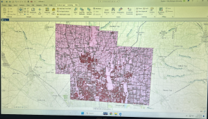
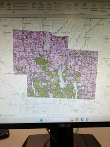
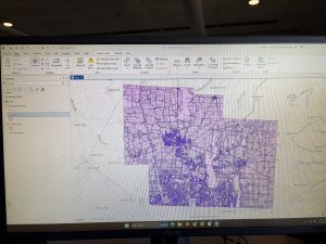
Inserted above is the image of my map after adding the three layers: Parcel, Street Centerline, and Hydrology

Zip Code: Contains all zip codes within Delaware County, Ohio. Published and updated monthly.

Street Centerline: Depict center of pavement of public and private roads within Delaware County, Ohio. Updated on a daily basis for all fields but the 3-D fields which are updated on an annual baiss, and is published monthly.

MASG: Stands for Master Street Address Guide, and is a representation of the 28 different political jurisdictions in Delaware County, Ohio.

Recorded Document: Consists of points that represent recorded documents in the Delaware County Recorder’s Plat Books, Cabinet/Slides and Instruments Records which are not represented by subdivision plats that are active. Documents such as; vacations, subdivisions, centerline surveys, surveys, annexations, and miscellaneous documents within Delaware County, Ohio. Updated on a weekly basis, and is published monthly.

Survey: A shapefile of a point coverage that represents surveys of land within Delaware County, Ohio. Surveys are found in documents in the Recorder’s office and the Map Department. The dataset is updated on a daily basis and is published monthly.

GPS: Identifies all GPS monuments that were established  in 1991 and 1997. Dataset is updated on an as-needed basis, and is published monthly.

Parcel: Consists of polygons that represent all cadastral parcel lines within Delaware County. Dataset is maintained on a daily basis, and is published monthly.

Subdivision: Consists of all subdivisions and condos recorded in the Delaware County Recorder’s office. The dataset is updated on a daily basis and is published on a monthly basis.

School District: The dataset consists of all School Districts within Delaware County, Ohio. The dataset is updated on an as-needed basis, and is published monthly.

Annexation: The dataset contains Delaware County’s annexations and conforming boundaries from 1853 to present. Dataset is updated on an as-needed basis once an annexation has been recorded within the Delaware County Recorder’s office. It is published monthly.

Township: The dataset consists of 19 different townships that make up Delaware County, Ohio. The dataset is updated on an as-needed basis and is published monthly.

Tax District: This dataset consists of all tax districts within Delaware County, Ohio. The data is defined by the Delaware County Auditor’s Real Estate Office, and data is dissolved on the Tax District code. The data is uploaded on an as-needed basis and is published monthly.

Address Point: A spatially accurate representation of all certfiied addresses within Delaware County, Ohio. The layer provides the capability to reverse geocode a set of coordinates to determine the closest valid address and is intended to provide 911 agencies with information needed to comply with Phase II 911 requirements. The dataset is updated on a daily basis, and is published once a month.

Municipality: The dataset contains the municipality parcels that are within the MSAG and Township datasets

Condo: Consists of all condominimum polygons within Delaware County, Ohio that have been recorded within the Delaware County Recorders Office.

Precincts: Consists of Voting Precincts within Delaware County, Ohio. Maintained by the Delaware County Auditor’s GIS Office under the direction of the Delaware County Board of Elections. Dataset is updated on an as-needed basis and is published as-needed by the Delaware County Board of Elections.

PLSS: Consists of all the Public Land Survey System (PLSS) polygons in both the US Military and the Virginia Military Survey Districts of Delaware County. Created to facilitate in identifying all of the PLSS and their boundaries in both US Military and Virginia Military Survey Districts of Delaware County. The dataset is maintained on an as-needed basis where new surveys have been recorded, dataset is updated on an as-needed basis and is published monthly.

Delaware County E911 Data: The database uses the Location Based Response System (LBRS) and is used in 911 Emergency Response. The dataset is updated on a daily basis, and is published monthly.

Farm Lot: Dataset consists of all the farmlots in both the US Military and the Virginia Military Survey Districts of Delaware County. Dataset was created to facilitate in identifying all of the farmlots and their boudnaries in both US Miltary and Virginia Military Survey Districts of Delaware County. Dataset is maintained on an as-needed basis where new surveys have been recorded.

Building Outline (2021, 2023, 2024): Consists of all building outlines in Delaware County. Each of the three databases are updated within their respective years.

Railroads: Allows a user to view the locations of railroads that lie within Delaware County.

Dedicated ROW: Consists of all lines that are designated Right-of-Way within Delaware County, Ohio. This data is line data that is created through the daily updates of Delaware County’s Parcel data. Dataset is updated on an as-needed basis, and is published monthly.

Original Township: Displays boundaries of Delaware County townships prior to divison by tax divisions affected their shape.

Map Sheet: Dataset contains all map sheets within Delaware County, Ohio. Consists of 360 records.

Hydrology: Dataset consists of all major waterways within Delaware County, Ohio. Data was enhanced in 2018 with LIDAR based data. The dataset is uploaded on an as-needed basis and is published monthly.

ROW: A type of easement (right-of-way) that shows accessible street routes in the form of line data.

2024 Aerial Imagery: 2024 3in Aerial Imagery Flown Spring 2024. Published on September 25, 2024 at 7:45 PM EDT.

Delaware County GIS Data Extract Web Map: Web map used in Delaware County GIS Data Extract application that allows users to extract Delaware County, Ohio GIS data in various formats.

2022 Leaf-On Imagery (SID File): 2022 Imagery 12in Resolution, published on September 14 2022 at 1:42PM EDT

Delaware County GIS Data Extract: Allows users to extract Delaware County, Ohio GIS data in various formats. Published June 8 2020 at 6:23 PM EDT.

Delaware County Contours: 2018 two foot contours for Delaware County, Ohio in file geodatabase format. Published April 9, 2020 at 9:51AM EDT.

Street Centerlines — DXF: The LBRS Street Centerlines depict the center of pavement of public and private roads in Delaware County, Ohio and was collected by field observation

Auditor Logo: The logo of the Auditor’s GIS Office in Delaware County

Fall Background: The background for different GIS data

Here is my map that shows all three layers: Street Centerline, Hydrology, and Parcles:

 

Cherry Blog week 5 

Chapter 4 

So far, which is quite honestly to be expected, is that the instructions and process of what we’re doing in GIS are getting progressively more complicated. I really struggled with the beginning of the chapter, where we were working with a lot of export files. I’d realized when I got past that part of the assignment, and I was unable to do something a few steps later, that I had done that completely wrong and had to essentially restart my project. 

This chapter altogether was a bit of a problem for me; I did learn quite a few new things regarding attribute tables and quite a few other things. I also liked seeing the crime data for 4-3 just because it looked interesting on the map. 

(My computer is broken, so I can’t access the screenshots from this section.) 

Chapter 5 

So far, the steps for Chapter 5 have been pretty easy, especially in comparison to Chapter 4. Besides doing different things with properties, there seems to be a lot of stuff that we have done previously, such as adding data or symbology stuff. 

Once I got to 5-5, where we were using Excel sheets, I was really confused, considering I’ve never worked with Excel sheets prior to this assignment, so it took me a lot longer than anticipated to do that section of the assignment. Although I was actually able to successfully import the information from the Excel sheet without too much trouble, that felt like a lot of accomplishment. I also feel like Excel is definitely something I will have to use in the future, so I am glad to get a little bit of experience using it. 

It was also interesting learning about what a Choropleth map is in more detail. I know we have worked with them quite a lot, but it was interesting to learn how we can join data alone to create one. 

 

 

Chapter 6 geoprocessing 

For this chapter and especially the 6-1 section, I actually quite liked learning how to work with the pairwise dissolve tool. It was kind of interesting to see the process and see the sectioning of the units turn into neighborhoods. Also, far through this chapter, I feel like I’m working on and going through the process of quite a few different new things, or at least things that weren’t significant enough previously to remember doing. Although getting to the end of 6-2, where I was trying to do your turn section. The selection by location was easy, but I keep getting confused on how to properly export some features, so I was struggling to save the selection under a different name. Overall, this chapter was quite a lot easier than the last two, so I was able to move smoothly through the post of the chapter with only a few hiccups, which is one of the first chapters I have been able to do so with so far with GIS. 

 

Chapter 7 

Chapter 7 was devoted entirely to editing existing features and creating new features, which turned out to be one of the most practical chapters so far in this tutorial. The tutorial has managed to cover a major portion of creating, moving, modifying, and deleting polygon features, which is quite different from what we have been doing so far in this tutorial.The chapter focused our attention on the fact that sometimes we, as GIS users, need to create our own spatial data. One of the most beneficial features of the tutorial is the use of the Modify Features pane, especially in choosing the vertices of specific buildings and making modifications to them as desired. We were taken through the tutorial step by step on how to utilize the Move, Rotate, Continue Feature, Reshape, and Split features, which showed us just how flexible ArcGIS Pro is, especially in making modifications to our features. We also learned the significance of precision in choosing our features because we need to be precise in choosing the feature that we would like to edit; otherwise, if we click slightly away from the feature, we may end up choosing the entire layer instead of the specific polygon. The most intriguing feature of the tutorial is the use of the smoothing edges feature. We learned how we can utilize the feature of smoothing edges on our features so that our features will be smoother instead of having jagged edges.Overall, this chapter helped me understand more about how GIS data is created, updated, and even corrected. I can definitely see myself using these tools again, particularly with any future assignments that require creating my own data or modifying data that already exists.

Chapter 8 

Chapter 8, like the last chapter, was short, and I feel like I have a much greater understanding of what geocoding is, particularly. It explained to me that geocoding is the process by which a set of location fields, such as street addresses or ZIP codes, is matched to the corresponding locations within a feature class. It also walked me through the steps necessary to use the ZIP code data, which is a simpler process, but then went on to explain how to use a full table of street addresses with an address locator. What I think this chapter did particularly well was to explain each part of the process within the Geo processing pane, making it easy to understand the relationship between the table, the locator, and the feature class. It also explained to me the importance of reviewing the addresses before geocoding to make sure they correlate with the locator. Should the addresses not correlate correctly, then the percentage of matches will decrease, resulting in a potentially incorrect outcome. It also showed how to view the matches once the geocoding is done. Another useful section for me was the part where I learned how to add the newly geocoded points to the map and visualize their distribution. While this chapter focused more on the process of creating the points, there was still a lot of emphasis on the importance of visualization when reviewing the results to spot possible errors. As this chapter used both ZIP codes and addresses, there was a distinction between coarse-level and fine-level geocoding. This will likely prove to be useful later on in the course, as accurate location information is the basis for almost all types of analysis. I can certainly foresee this chapter proving useful to me when working on the final project or any assignment with a table that includes spatial data.

Chapter 9 

Chapter 9 described one of the most used GIS tool types; buffer analysis. This chapter is one of the longer and more detailed ones because there are many ways of proximity measurement with geo processing tools. The chapter began with a tutorial on how to create a basic buffer around a feature at a specified distance and how the result differs when features are dissolved or not. The chapter also taught how to create multi-ring buffers and how to visualize data at different levels of proximity. This was a good approach to understanding how proximity affects data from a point or a polygon feature. The chapter also taught how to use various tools in the Geo processing pane. The chapter was also good at emphasizing the importance of setting input layers, choosing output locations, and making sure all parameters are filled out when running a tool. The chapter was also good at emphasizing the importance of keeping track of geo databases so that output layers are not lost, which can easily happen. What I thought was most interesting was how this chapter taught how buffers are a fundamental tool in many real-world analyses, including the ones in this chapter. The chapter taught how proximity could be used as a tool for analyzing and understanding different types of analyses, such as creating zones, finding areas of interest, and preparing for later network analyses. Although this chapter did not go in-depth with network analyses, it did show how buffers are a subset of this type of spatial analysis. Chapter 9 gave me a better understanding of spatial relationships and how to create meaningful proximity layers with the buffer tool in ArcGIS Pro.

 

 

Zip Code: All zip codes within Delaware County, and is updated and published monthly. 

Street Centerline: The center of pavement of public and private roads in Delaware County, updated annually and published monthly. 

MASG: Master Street Address Guide, represents the 28 different political jurisdictions in Delaware County. 

Recorded Document: Points that represent recorded miscellaneous documents in Delaware County, it is updated weekly and published monthly. 

Survey: Point coverage that represents surveys of land in Delaware County, it is updated daily and published monthly. 

GPS: All GPS monuments that were established in 1991 and 1997, it is updated as needed and published monthly. 

Parcel: Polygons that represent all cadastral (used for taxation) parcel lines in Delaware County, it is maintained on a daily basis and is published monthly. 

Subdivision: All subdivisions and condos recorded in Delaware County, it is updated daily and published monthly. 

School District: All the school districts in Delaware County, and is updated as needed and published monthly. 

Annexation: Delaware County’s annexations and conforming boundaries from 1853 to present, and is updated as needed once an annexation has been recorded, and is updated monthly. 

Township: Consists of the 19 townships that make up Delaware County, and is updated as needed and published monthly. 

Tax District: All the tax districts in Delaware County, and is defined by the auditor’s real estate office. It is updated as needed and published monthly. 

Address Point: Spatially accurate representation of all the certified addresses within Delaware County, and it is updated daily and published monthly. 

Municipality: All municipalities in Delaware County. 

Condo: All condominium polygons in Delaware County that have been recorded. 

Precincts: All of the voting precincts in Delaware County, it is updated as needed and published by the Delaware County Board of Elections. 

PLSS: Public Land Survey System polygons for both the US Military and the Virginia Military Survey Districts, and is updated as needed and published monthly. 

Delaware County E911 Data: The State of Ohio Location Based Response System has a spatially accurate representation of all certified addresses in Delaware County, and it is updated daily and published monthly. 

Farm Lot: All the farmlots in US Military and Virginia Military Survey Districts of Delaware County, updated as needed where the new surveys have been recorded. 

Building Outline 2023: All of the Building Outlines from 2023. 

Railroads: The locations of all the railroads in Delaware County. 

Dedicated ROW: All lines that are designated Right-Of-Way within Delaware County, it is updated daily and published monthly. 

Original Township: The original boundaries of the townships in Delaware County before they were affected by tax district changes. 

Building Outline 2021: The building outlines for all structures in Delaware County and is updated on an as needed basis. 

Map Sheet: All map sheets within Delaware County. 

Hydrology: All major waterways in Delaware County, it is updated as needed and published monthly. 

ROW: All lines that are designated Right-Of-Way within Delaware County, it is updated as needed and published monthly. 

2024 Aerial Imagery: Aerial images from 2024 of Delaware County. 

Delaware County GIS Data Extract Web Map: Allows users to extract Delaware County GIS information in different formats. 

2022 Leaf-On Imagery (SID File): 2022 imagery 12in resolution. 

Delaware County GIS Data Extract: Allows users to extract Delaware County GIS data. 

Address Points – DXF: The LBRS Address Points data provides a spatially accurate placement of addresses within a given parcel, and is updated as needed. 

Delaware County Contours: 2018 Two Foot contours for Delaware County. 

2021 Imagery (SID File): Images of Delaware County from 2021. 

Street Centerlines – DXF: The LBRS Street Centerlines depict the center of pavement of public and private roads in Delaware County, and was collected by field observation. 

Building Outlines – DXF: An image of the building outlines in Delaware County. 

Auditor Logo: The logo of the Auditor’s GIS Office in Delaware County. 

Fall Background: The background for different GIS data. 

Building Outline 2024: The outlines of buildings in Delaware County from 2024. 

 

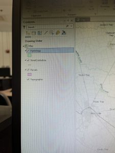
I put the Hydrology layer on top of the Parcel and StreetCenterline so I could actually see it. The Add Data feature was very helpful in this, and I have attached my map and an image of my catalog pane.

Chapter 4: Mapping Density

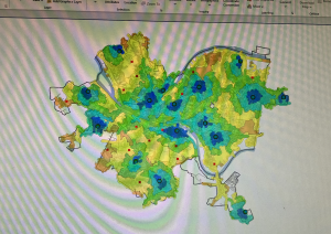
This chapter mostly focused on what a density surface is and how GIS takes point or line data, like businesses, roads, or population centroids, and turns it into a smooth surface that shows where things are more concentrated. The chapter explains that cell size really matters because smaller cells show more detail but take longer to process, while larger cells make the patterns more general and can hide smaller variations. I also learned about search radius, which is basically how far the GIS looks around each cell when calculating density. A smaller search radius shows more local differences, but if it is too small, broader patterns might not show up. A larger search radius smooths everything out and shows bigger trends, but it can also blur details that might matter. Another important idea is that GIS can calculate density using simple or weighted methods, where the weighted method gives more importance to features closer to the center of the search area and usually creates smoother and easier to read maps. The chapter also talks about choosing the right units for density, like per square mile or per acre, and how using very large units can make density values seem misleading even if the overall pattern stays the same.
It was also very interesting to learn how much control you actually have over the patterns you end up seeing. Just changing the cell size or the search radius can completely change how the map looks, even when the data itself doesn’t change at all. The examples showing how patterns become too blocky with large cells, or too smoothed out with a big search radius, makes it clear that there is not really one “correct” setting. It depends on what kind of pattern you are trying to understand. Another thing that I noticed was that the highest density area on a map does not always mean something is actually located there, since density is calculated based on nearby features. That made me realize that density maps are more about showing general patterns than exact locations.

Chapter 5: Finding What’s Inside

Some of the key things I picked up from this chapter were how GIS is used to figure out what falls inside certain areas and how that helps compare places in a more meaningful way. The chapter explains that you can do this in a few ways: sometimes you can just draw the boundary on top of features to visually see what is inside, sometimes you select the features inside an area to get a list or count, and other times you actually overlay layers to measure what is inside each area. This makes it possible to answer questions like how much forest is inside each watershed, which parcels fall at least partly inside a floodplain, or how many roads run through a protected area. It also talks about vector and raster overlay, where vector overlay is more precise but slower and can create small and messy pieces called slivers, while raster overlay is usually faster and avoids slivers but depends a lot on cell size for accuracy.
Another thing that I found important was how the type of data changes what kind of summary you can get at the end. When working with categories, like land cover types, you can summarize how much of each category is inside an area and even convert it into percentages to compare areas fairly. When working with continuous data, like elevation or precipitation, GIS calculates statistics such as the mean, minimum, maximum, range, or standard deviation for each area. The chapter also shows how results end up in tables that can be joined back to maps, which makes it easier to compare areas visually instead of just guessing from the map.
It also made me think about how often people use this kind of analysis without realizing it, like when cities decide where to put new services or when environmental groups compare protected areas. It makes me curious about what kinds of “what’s inside” questions are most common in real GIS jobs.

Chapter 6: Finding What’s Nearby

This chapter helped me understand what “nearby” actually means in GIS and how GIS can define it in different ways depending on what you actually mean by near. Sometimes it is just straight-line distance, and sometimes it is just about travel range, like what is within a 3-minute drive of a fire station. This chapter explains that “near” can be measured by distance, but it can also be measured by cost, especially time. It also introduces three main approaches, which are: using straight-line distance, measuring distance or cost over a network (like streets), and calculating cost over a surface for overland travel. I also learned about details that can change results, like planar vs geodesic distance (flat vs curved Earth) and the difference between inclusive rings and distinct bands when you need multiple distance ranges.
As always, I have found this very important to know how much the method you choose can change the story the map tells, even if the starting point is the same. For example, a circle around a store might be fine for a rough estimate, but it is not the same as a real 15-minute drive because streets, turns, traffic, and one-way roads can shape how people actually move. This chapter makes that really clear with the network examples, especially when it talks about assigning “impedance” to street segments using distance, time, or money. I also liked the idea that you can build more realistic travel time by adding turn and stop costs using a turntable, because that is the kind of small detail that matters a lot for something like emergency response. And I didn’t realize there were so many output options like buffers, selections, point-to-point distances, spider diagrams, distance surfaces, and service area boundaries like (compact vs general) depending on what you are trying to show.
If someone uses straight-line distance for something that really depends on travel time, the results can be misleading, especially in places with rivers, highways, or weird street layouts. That made me wonder how GIS people deal with real projects when the data isn’t always perfect. Like, if you don’t have exact speed limits, turn delays, or updated road closures, how do you decide what’s “good enough” without making the map seem more accurate than it actually is?

Data Inventory:

Zip Code: Contains all of the zip codes that fall (either completely or partially) within Delaware County. These parcels were created in 2005 according to property addresses, likely to ensure that properties were not split across zip codes.

Street Centerline: This data depicts the center of the pavement of all public and private roads in Delaware County to give a fair approximation of street routes throughout the county. This street system is called the Ohio Location-Based Response System (LBRS) and is heavily used by ODOT and emergency services. Street segments are measured from vertex to vertex.

MSAG: The Master Street Address Guide (MSAG) delineates townships and municipalities in Delaware County. Most townships are simple geometric rectangles, but the municipalities are irregularly shaped. Some municipalities are also their own townships, and they are located inside of other townships, as is the case with Sunbury Township located inside of Berkshire Township.

Recorded Document: These are records that do not match up with the subdivisions that currently exist on the Delaware County map. They include records of vacations, cemeteries, road centerline surveys, and utilities easements.

Survey: This dataset is a collection of the locations of all recorded land surveys in Delaware County more recent than Old Survey Volumes 1-11. There is a pretty high density of land surveys all throughout the county, except over bodies of water and in parks like Alum Creek State Park, Delaware State Park, and the Dover Recreation Area.

GPS: This dataset displays the shapefile of GPS monuments, or metal disks in the ground that mark latitude and longitude and serve as reference points. These monuments were established between 1991 and 1997. 

Parcel: This dataset is incredibly detailed, showing land parcels in Delaware by ownership. Contains extensive information on each property, such as the address, current owner, sale history, and number of rooms.

Subdivision: This dataset contains subdivisions and condos in Delaware County. (These types of housing are typically higher-density residential areas.) Most subdivisions appear to be concentrated around the town of Delaware or the southern part of the county.

School District: All the school districts in Delaware County are displayed in this data set. Similar to the Zip Code data set, some small portions of school districts that mostly fall within adjacent counties are included.

Tax District: The tax district dataset appears to line up similarly to the MSAG data set but includes a few more divisions. Most of the tax districts around municipalities are shaped irregularly and are even sometimes nested shapes within the more geometric townships.

Annexation: This dataset shows annexations in Delaware County. They are concentrated around towns like Delaware, Sunbury, Powell, and Westerville.

Township: Shows all of the townships in Delaware County. Very similar to the MSAG dataset.

Address Point: This dataset uses LBRS to show all registered addresses in a shapefile. The point on the map is located in the centroid of the building.

Municipality: This dataset contains the municipality parcels that are noticeable in the MSAG and Township datasets.

Condo: Condo polygons are shown in this dataset. They are pretty small and well-dispersed, which, when compared to the Subdivision dataset, leads me to believe that Delaware County has lots more houses in subdivisions than condos.

Precincts: Delaware County voting precincts line up pretty well with township and municipality parcels but are divided within into much smaller areas.

PLSS: This dataset contains Public Land Survey System (PLSS) polygons, most of which are near perfect squares. However, the west side of Delaware County comprises more irregular PLSS polygons.

Delaware County E911 Data: This dataset uses an LBRS system of Address Points and is used in particular by 911 Emergency Services. Other uses include appraisal mapping, geocoding, reporting accidents, and managing disasters. This is measured in terms of US Military and Virginia Military Survey Districts.

Farm Lot: Contains all farm lots (as measured by military districts). Many are different shapes: square, long and thin, uniform rectangular, or irregular (as in the western and central parts of the county).

Building Outline (2021, 2023, 2024): Contains all building outlines in Delaware County. Very reminiscent of a Google Maps view. Each of the three databases was updated in its respective year.

Dedicated ROW: ROW stands for Right-of-Way, which is a type of easement, so it shows accessible street routes in the form of line data. It appears that streets that are not included as ROW routes are in private subdivisions or similar areas.

Railroads: The dataset highlights railroads running through Delaware County, and it appears that most of them run north-south.

Original Township: Displays boundaries of Delaware County townships prior to division by tax districts. Consists of 18 original townships. The eastern portion of the county has rectangular parcels, and the western portion’s parcels are more irregularly shaped, which is consistent with other similar datasets.

Map Sheet: A map sheet is just a map that is part of a larger map series. The data appears to show data at the sub-municipality or sub-township level. The smallest parcels are clustered around the cities of Delaware and Sunbury, and in the southern portion of Delaware County.

Hydrology: Contains the portions of all *major* waterways in Delaware County. Many small ponds and lakes on the map do not appear to be counted in this dataset.

ROW: Just like the Dedicated ROW dataset, this contains all line data of street rights-of-way in Delaware County.

Delaware County Contours: Contains two-foot contours showing the topography of Delaware County. This data was updated in 2018. It is in the form of a downloadable geodatabase.

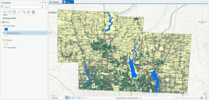
Map:

Figure 1: Delaware County Parcels (yellow), Street Centerline (green), and Hydrology (blue) layers.

Once I remembered I had to use the Add Folder button to add my files into the Catalog pane, it was smooth sailing making this map!

 

 

chapter 7

I enjoyed completing chapter 7, especially the first few tutorials, where I got to just move around and adjust the outlines of buildings and correct them. It was fun to do but it also made a lot of sense. I liked that there were only 4 in this one, I was able to take in each tutorial really fast and go back through to make sure I fully understood. I actually really enjoyed doing these ones because I have gotten much more accustomed to all the contols like adding features, symbols, bookmarks, and the repetitive tabs.

chapter 8

It was really easy to do these ones, considering it was only 2 tutorials, but I still feel like I gained a lot from them and got valuable knowledge on Geocoding and analyzing locations, plus learning about things with zipcodes. Most of the infomation was stuff I had begun to feel confident with, doing things with the creating locator, for example, went smoothly. When rematching attendees by zipcode on 8-2 I got a bit lost at a certain part where I had to click the match button for the zipcodes, for some reason it wouldn’t load for me. Also, the create locator section kept resetting on me and deleting my data.

chapter 9

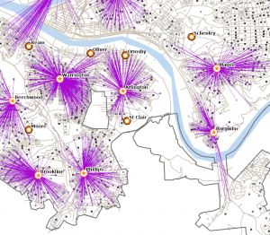
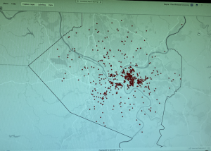
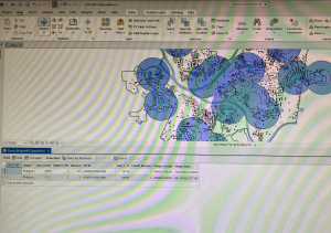
This one had the most tutorials technically but it still wasnt a long time to get through. Buffers were something I had been confused on before too, so i liked being reintroduced to this chapter. I know you use them to find whats near the features being buffered, but seeing them in action helped a lot. 9-1 and 9-2 on the swimming pools in Pittsburgh and estimating the number of youths was really quick and easy. I also thought it was cool how it highlighted the ones within half a mile. I also thought the dissolve option was really neat, helping with overlapping buffer rings helps make it much better to look at.

9-3 it estimates gravity models of geography, you can see the amount of attraction between two features. I had trouble figuring this part out, it was probably the hardest for me out of all the units. It wasnt that bad but I kept getting stuck at the parts where it would ask me to click the service area layer, it would genuinely not give me what I needed, it took me a second to try and figure out how to get through these tutorials at the end but it was still cool. I think analyzing the optimal soltuions and doing your turn was difficult, but it was also a pretty informative.

 

 

 

 

 

 

Chapter 7

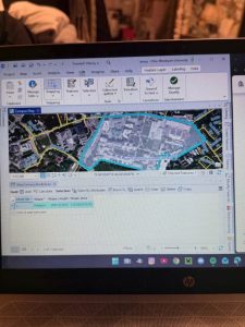
Chapter 7 introduced the practical processes involved in editing and creating spatial data. It emphasizes that GIS is not simply about viewing maps but also actively maintaining them as well. Through moving and reshaping polygon features of the campus, it became clear to me that spatial data must continuously evolve. The ability to edit vertices and create new feature classes such as parking lots and bus stops seemed quite interesting to me. I found applying the Smooth Polygon tool to be easy and the end result of it aesthetically pleasing. 

Chapter 8

Chapter 8 explored the process of geocoding, which connects tabular data such as addresses and zip codes to geographic locations on a map. The only part I found interesting in this reading was the process of reviewing matched and unmatched records – was almost like a puzzle. It demonstrated that GIS analysis depends not only on automated tools but also on critical evaluation. This chapter emphasized that spatial accuracy directly influences the validity of conclusions drawn from mapped data. The consequences of having incorrect mapped data could affect overall public safety, or even service delivery. Moving on, the buffer analysis tutorial around public swimming pools in Pittsburgh taught me how juxtaposition plays a role in accessibility. This idea particularly applies to youths living within a half-mile radius of recreational facilities – in other words, the pools.

Chapter 9

This last chapter focused mainly on spatial analysis, specifically showing how GIS can move beyond simple mapping. Using buffer tools around public swimming pools in Pittsburgh, I calculated how many youths live within a half-mile of a pool. Afterwards, I calculated what percentage of the city’s youth population that represents (I am thankful I don’t have to do actual calculations. This made the concept of accessibility much more believable, especially when thinking about how distance affects whether someone will realistically use a public facility. With this in mind, I can see how it is important to look at maps such as this in order to acquire the most efficient spot for a public facility.  It also became clear that straight-line buffers do not always reflect real travel conditions. It is not accurate when terrain and bridges are not included. My thoughts for this chapter include knowledge of how GIS can support planning decisions, such as which public restrooms to shut down because of low funds. It is advantageous because it can turn spatial data into measurable series, ones you can apply to real-word problems. 

 

7:

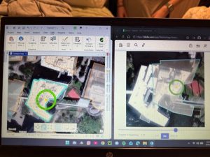
     In chapter seven, we learned how to edit polygon features as well as how to use specific tools to directly depict these features. I really enjoyed chapter 7 as it reminded me of working with vectors in Adobe Illustrator, where you can adjust shapes using various tools and vertex points. When creating polygon features, I found the trace tool very satisfying to use. Learning how to smooth out the edges of the polygon was also very satisfying. I also found it interesting that when the chapter was teaching us how to transform features, it used an AutoCAD drawing as a base to transform. Until now, I had no clue that AutoCAD could be utilized by ArcGIS, as I am semi-familiar with AutoCAD software. In chapter 7, it also says we can click and hold the wheel button on our mouse in order to pan around the map when in editing mode. This was helpful information that I wish the book had told us when making feature edits earlier. 

8:

        Chapter eight was more confusing than the previous chapter for me. It has to do with geocoding, which is the ability to convert various geographic data descriptions/addresses into geographic coordinates that can be displayed on a map. To be specific to chapter 8, it taught us to geocode using zip codes and street centerlines. These actions that allow for geocoding are done mostly through the use of specific tools found in the Geoprocessing pane. Throughout the later tutorials, sometimes they dont actually say “run tool” when that step needs to be conducted. I guess it can be assumed that the tool needs to be run, but I prefer tutorials that are very detailed and explicit in their instructions. This was a small detail, but it made the workflow feel slightly less clear and more frustrating at times. It also doesn’t help that you don’t get a visual on what you’re imputing until the very end of the imput.

 

9:

        I ended up understanding the concepts from chapter nine much better than in chapter eight. With the concept being how to work with/display spatial data, which is (to my understanding) the area surrounding a data point that can be utilized to answer specific questions. For example, we created service areas to help compare how often a pool is used by youths depending on the travel time to said pool. The travel time is visualized by the service areas as ring boundaries around the pool data point. As expected, the use rate of the pool was decided as travel time went up. I also may have found this chapter easier because, unlike the previous chapter, you could visually see the map changing as you performed each little step.