Chapter 1
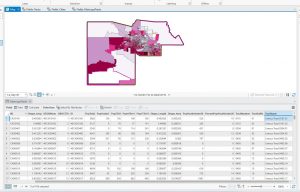
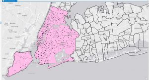
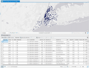
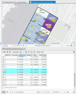
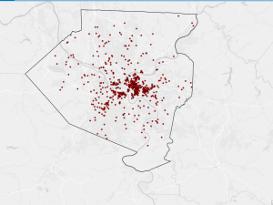
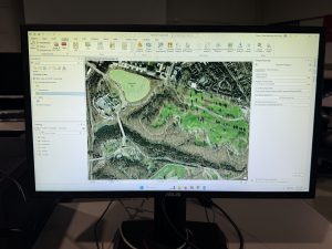
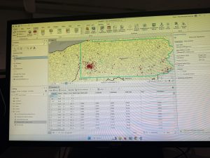
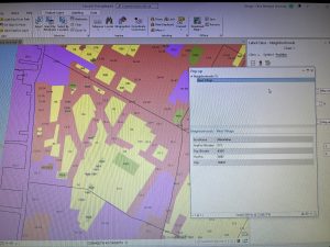
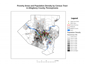
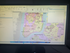
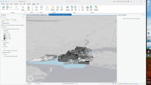
To start this assignment, I like how the tutorial book explains how each button you click changes the map in a specific way and you can see the differences. I appreciate how straightforward they are in explaining each step of viewing the maps. As I went on, tutorials 1-2 explained the movement and navigation programs. I appreciated that one false move wasn’t going to ruin my entire progress as the undo button became my best friend several times. I was able to better understand where everything was within ArcGIS. When it came to tutorial 3, I started to work with actual data points. I was able to pull up different statistics and look at an attribute table. As well as edit it for different reasons and look at the summary statistics. Tutorial 4 I had some initial issues pulling up the symbology for the FQHC clinics but I just didn’t have the valid data source on the layer. Once I got that hiccup dealt with I had no issues with the rest of Chapter 1 practice with 3D maps.
Chapter 2
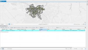
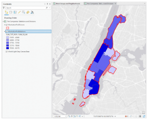
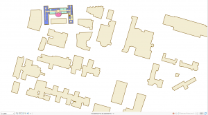
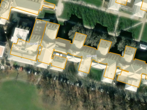
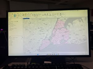
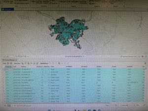
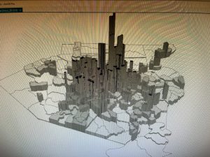
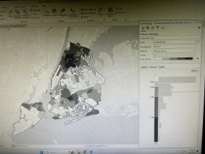
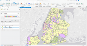
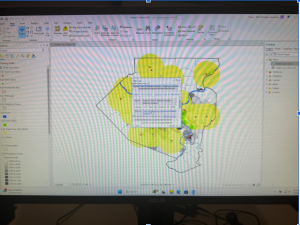
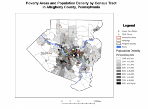
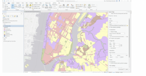
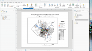
I took my time with this chapter since it was a bit more challenging. I enjoyed working on symbolizing maps and creating custom scales to suit my needs. The most confusing part for me was deciding which methods to use for choropleth maps. It seems like you really need to grasp statistical concepts, like data distribution, to make the right choice. I’m worried that when I start working with my own data, I might struggle to pick the most suitable scales for the best results. Another tricky part was the definition query, mostly because I’m not very tech-savvy, so it was a bit outside my comfort zone. However, I did learn some useful skills, like how to remove duplicate labels, adjust font sizes and colors, and explore more advanced 3D map features. One feature I found especially interesting was the Visibility Range option for feature layers. It allows a layer to appear or disappear depending on the zoom level, which helps make maps less cluttered and easier to navigate by only showing data when it’s at the right zoom level.
Chapter 3
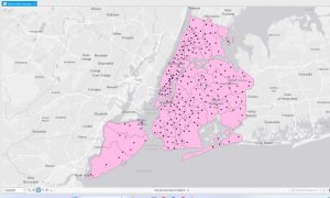
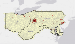
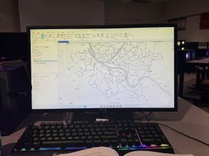
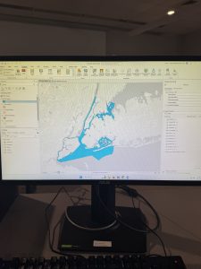
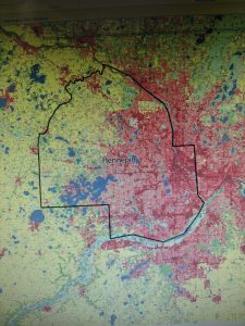
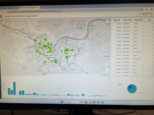
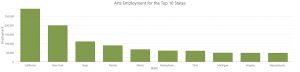
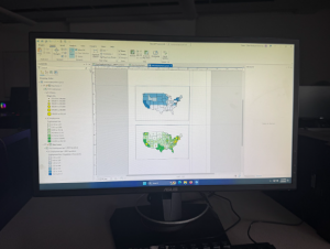
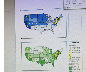
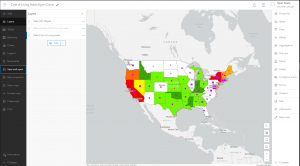
It began by teaching map layout techniques, including adding legends, using the ruler to align elements, and exporting maps. These skills felt especially useful for creating educational maps or preparing professional presentations. The chapter also covered how to create charts based on map data, like a graph that focused on the employment statistics of just 10 states, making it easier to visualize trends without being overwhelmed by a larger dataset. The tutorial then shifted to ArcGIS Online, where I learned how to share maps and create StoryMaps. While I had some experience with ArcGIS Online, there was still a bit of a learning curve. It seemed intuitive and user-friendly but lacked some of the advanced features of ArcGIS Pro. Creating a StoryMap was fun, though it would’ve been even better to use my own words and data instead of just copying and pasting. Overall, the chapter gave me valuable experience using ArcGIS Online to create interactive maps and reach a wider audience with visually appealing presentations.