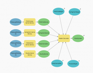
Chapter 4
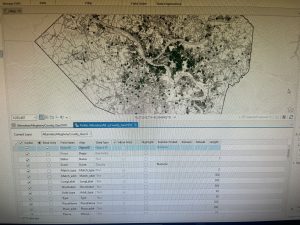
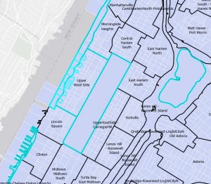
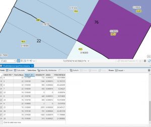
This unit was more difficult as the instructions didn’t involve much detail, and I had to remember many procedures from previous chapters. In Tutorial 4-1, I created a new ArcGIS Pro project named “YouthPopulation” and connected external folders, allowing access to spatial data. Converting shapefiles to feature classes reinforced the importance of proper file organization. Tutorial 4-2 involved modifying attribute tables, deleting unnecessary columns, and renaming fields, but I accidentally skipped the “Your Turn” section, which required creating the Tract feature class. This mistake forced me to redo the tutorial, reinforcing the importance of completing all exercises. In Tutorial 4-3, the SQL syntax was challenging, but ArcGIS Pro’s query builder helped. Tutorial 4-4 introduced spatial joins to aggregate burglaries by neighborhood, emphasizing data organization. In Tutorial 4-5, I learned how to create central points from polygons using the “Feature to Point” tool and the “Calculate Geometry” tool to add coordinates. The distinction between centroids and central points was particularly useful. Tutorials 4-6 covered creating a code table for crime hierarchy codes and performing a one-to-many join for better data representation. Managing these joins and understanding the limitations of large datasets were key takeaways. 


Chapter 5
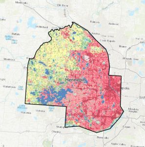
This chapter focused on projections, coordinate systems, and working with U.S. Census data, making it a more technical and detail-oriented unit.. Tutorial 5-2 highlighted the importance of selecting the correct coordinate system early on, as it impacts later analyses. Working with external geospatial data and understanding how different formats interact with ArcGIS Pro was a valuable experience, the need for precision in GIS workflows was proved to me again from this chapter. By the end of the chapter, I had a stronger understanding of how projections influence spatial accuracy and how to effectively prepare datasets for mapping and analysis. This unit served as a great reminder of how foundational GIS concepts come together in practical applications.

Chapter 6
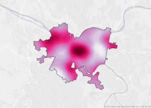
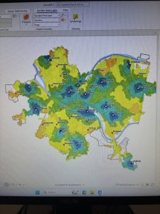
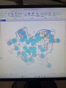
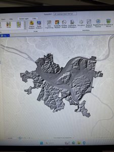
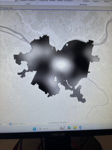
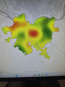
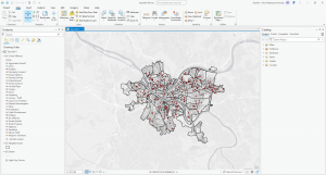
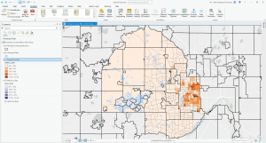
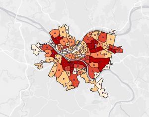
Chapter 6 focused on geoprocessing techniques such as dissolving features, extracting and clipping study areas, and merging layers, for mapping fire company zones in Manhattan. A key task involved using the Pairwise Dissolve tool to group fire companies into battalions. In the beginning, I didn’t understand what the point of this tool was, after using it and experimenting for a bit I got what it is about. Fire battalions were symbolized using graduated colors to represent population density. Using graduated colors gave useful information to the map, and the different densities are easy to tell apart with this feature. Labeling the fire battalions was the most challenging part, as it required working with label properties to ensure the names and numbers were displayed correctly without cluttering the map and making it hard to read.

Chapter 7
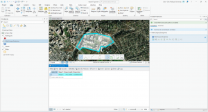
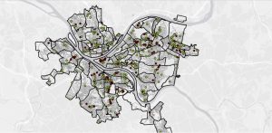
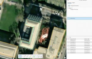
Chapter 7 introduced digitizing techniques, focusing on editing, creating, and transforming polygon features in ArcGIS Pro. This unit involved various tools and methods to manipulate spatial data, such as modifying existing polygon features, adding new ones. One of the key things I learned was working with tools that enhance the visual representation of geographic features, along with spatial transformations. A particularly challenging part was figuring out how to use the Split tool effectively, as it required precision in dividing features correctly while maintaining the integrity of the dataset. Unlike previous chapters, this unit required a more direct interaction with the features rather than simply applying geoprocessing tools. The experience was engaging and I liked it.

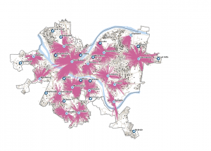
Chapter 8
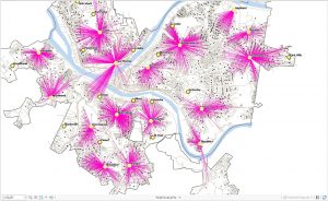
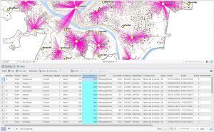
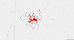
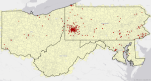
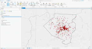
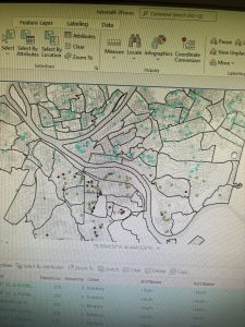
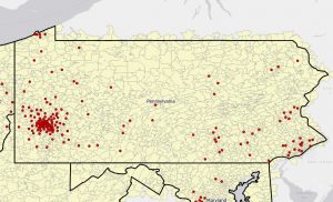
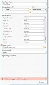
Chapter 8 introduced geocoding, which focused on converting addresses and zip codes into mappable points, making it one of the more practical and engaging topics so far. This unit involved working with both zip codes and street addresses to analyze spatial data, which was interesting because it showed how location-based information can be transformed into meaningful insights. I found the process of matching addresses to locations straightforward, especially after getting used to ArcGIS Pro’s handling of data inconsistencies. Unlike previous chapters, nothing in this unit felt overwhelmingly difficult—I’ve started to adjust to the workflow and feel more comfortable navigating the tools. The matching techniques for improving address accuracy were particularly useful, and it was satisfying to see how geocoding could be applied to real-world scenarios, like analyzing event attendance based on survey data. Overall, this chapter reinforced how GIS can make spatial data more practical and accessible, and it felt like a natural progression in applying everything I’ve learned so far.