4-1: For the section “Use database utilities in the catalog pane”, I was unable to do the copy and paste sections from part 2 and 3, paste just wasn’t showing up for me. I was able to finish the rest of the section, and since it asked you to delete everything at the end, it ultimately didn’t matter.
 Screenshot (22).png
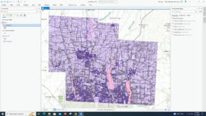
4-2: Tracts was not in my contents page for some reason. I ended up going to the catalog pane, to folders, and right clicking tracks to add it t0 the map. Showed up on my contents page then. Hope that’s right. Actually, for delete unneeded columns, my table did not end up looking like the one in the book, instead of fully deleting even though I clicked it all the unneeded columns were just in a lighter gray. Because of this, I was completely unable to finish the section. And it was a long section.
Screenshot (23).png
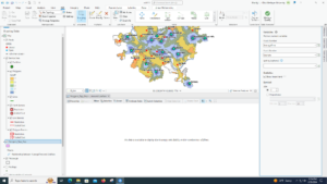
4-3: After I was doing the section correctly, I opened the crime offenses attribute table and when there should’ve been 444 remaining features, there was still 3924. My SQL expression looked like the one in the book, so I do not know why this happened. At the end of the tutorial, I ended up with two people instead of just one too.
Screenshot (24).png
4-4: This was a short tutorial and one I was able to do 100% successfully, thank god.
4-5: This tutorial was also short and I had no problems with.
4-6: Same as the last 2 tutorials. The latter half of the 4 tutorials were a lot easier than the first half.
5-1: I had no idea there were around 5200 projected coordinate systems and over 100 map projections. How would you even know what’s best for what you’re trying to do?
5-2: Again, there are so many coordinate systems and map projections.
5-3: This one was interesting. I don’t really understand why I was changing the projected coordinate systems and why this matters so much.
5-4: CouncilDistricts was not in my Chapter5,gbd, so I used municipalities because it seemed close enough. I also did not have libraries in it.
Screenshot (28).png
5-5: This tutorial is really confusing. Column JK, which I was supposed to keep, was not the same as what the book said it should be- it was females not living in a place. And there was no column SE at all, so I was unable to do this section. When moving to the next section, I was unable to find most of the census shapefiles and I am not sure why. Because I couldn’t do this, I couldn’t do the next section. So I pretty much was unable to do this entire tutorial except downloading the data at the beginning.
Screenshot (30).png
5-6: Eliminating the land use for everything else other than just the county is interesting. Actually looking at the data is really cool though, and seeing the difference in development. Also, ground features wasn’t an option to symbolize the elevated contours layer for me, so I just changed the color to a similar one instead. I am not the biggest fan of the textbook assuming we know how to do everything we previously learned 100% perfect, as I don’t have the best memory.
6-1: This one was fairly easy and makes sense why this would be useful.
6-2: I am unsure of how to export the selected features as UpperWestSideBlockGroups to Chapter6.gdb. Also, I couldn’t find UpperWestSideStreetsForGeocoding, so I couldn’t clip streets either.
Screenshot (40).png Screenshot (41).png
6-3: This tutorial seems really useful. Being able to combine all that data and clear up the contents page makes for much easier map readability.
6-4: Pretty much the same as the last tutorial. I have the same thoughts on it too.
6-5: I do not see SUM_Street_Length in my attributes table, only Street_Length. I’m pretty sure I did this section right so I’m not sure why it’s not appearing for me, even when the table is refreshed
Screenshot (44).png
6-6: I don’t think I joined the tables right at the end. I didn’t really see how I could do it, clicked around and found something called join, but got a lot of null sections. I wish the book could explain in more detail how to do some steps, because even though it’s later on in the book there’s so much information that its hard to remember it all.
Screenshot (45).png
6-7: I liked the background behind this tutorial. It reminds me that GIS is used for really important and possibly life-changing information, like separating the disabled people in half between 2 fire companies so in the heat of the moment no one gets left behind because of not remembering.
7-1: I don’t know where a constructions toolbar is, so I couldn’t click the add button and move the vertex points of the art building. I had issues with splitting the buildings too, but this is probably just a me thing.
Screenshot (47).png
7-2: It took me awhile to do this tutorial, as working with these polygons was finicky for me, but I eventually was able to do everything in the tutorial.
7-3: Well this tutorial was easy. I can understand how smoothing out the polygons can help with viewer comprehension.
7-4: I feel like this is something I would never remember how to do. It looks pretty cool though.
8-1: For me, the rematch addresses pane doesn’t have a “pick from the map button”, so I couldn’t finish the “rematch attendee data by zip code” section. The next section, “symbolize using the collect events tool” didn’t work for me either, as when I tried to run the tool I kept getting “collect events failed” multiple times, even with changing some things up.
Screenshot (50).png
8-2: My only issue with this tutorial is that the basemap, World Light Gray Canvas Base, didn’t load for some reason. Otherwise this one made sense.
Screenshot (51).png

 I got a couple error messages when I tried right click UseRate and clicked Calculate Field. I’m assuming it’s because I typed in the expression wrong, maybe I put spaces when I shouldn’t have. I believe this inhibited me from making a scatterplot, as when I typed in the X and Y axis fields, there was no button to apply or even in the Edit tab i wasn’t able to save. So I was unable to completely finish the project.
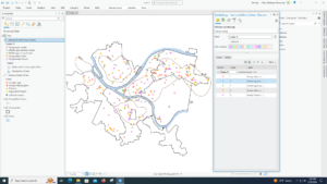 I liked the background of this tutorial. Mapping crimes, especially violent ones, are really important and its cool to see in real time how you can define the data to make it more understandable.
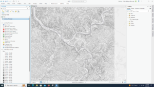 I don’t have “LandUse_Pgh” in my files, only “LandUse_Pgh.tif”. So, I have the land use for a good distance around pittsburgh instead of just the city itself. Actually, another time I tried to find it in the geoprocessing pane it was there. Sometimes files just don’t show up for me. I also don’t have NED_Pittsburgh, just NED. In the end, my tutorial looks just like the one from the book, except the Pittsburgh outline disappeared somewhere along the way and everything I did to the map didn’t just go inside the Pittsburgh limits.
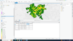 I thought that this tutorial was interesting. Learning how to make a heat map seems pretty cool.
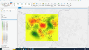 This tutorial was really long for me. I was able to do it all though, except for the fact that the poverty index model goes outside the Pittsburgh borders. Not sure why that happens to me so much. This was really complicated but seems useful.
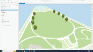 I don’t see the “Get Z From View” button. I also don’t have the cute trees the book has but it is a fun tool to know.
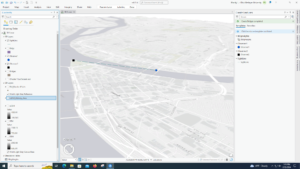 This tutorial was also interesting to do. Creating the buildings out of thin air was cool. I definitely messed up somewhere along the way though because I didn’t get the proper sightline at the end.
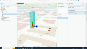 Not too sure how many uses these tools have, other than scale I guess.
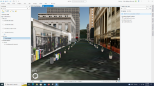 This tutorial was super fun. The end product, the Smithfield street 3D, was cool to explore and the little planters, trash cans, and fire hydrants were cute.