Chapter 7:
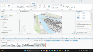
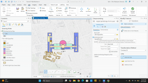
This chapter talks about digitizing. There are a wide variety of tools that are available when editing and creating GIS features. In this chapter, the tools introduced are used for manual digitization by tracing. Base maps are used to learn how to edit and create vector features. The chapter also discusses the creation of new feature classes and the use of base maps or existing layers as spatial guides in the digitization of features. Lidar is also used as a reference for heads-up digitizing. Vector features can be created using GPS receivers that collect longitude and latitude data. CAD and building information modeling (BIM) files can be imported into GIS maps and can be used to create feature classes.
Tutorial: in this chapter, it shows:
- Edit polygon features
- Move features
- Rotate features
- Add and remove vertex points
- Split features
- Create and delete polygon features
- Add a feature class and create polygons
- Delete polygons
- Use the trace tool to create a polygon feature
- Use cartography tools
- Smooth a green space polygon
- Transform features
- Add a CAD drawing and view layers
- Use geo reference to move and rotate CAD drawing
- Export the CAD file and assign a projection
- Explore attributes and classify layers
- Transform polygons
This chapter was very helpful in showing how to move and rotate buildings to line them up with the base maps. This chapter did a good job, in my opinion, of showing how easy it can be to digitize map features and align external information to GIS.
Chapter 8:
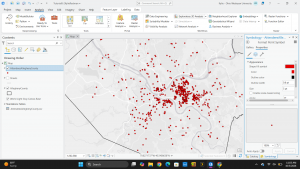
This chapter explains how to geocode address data and create point features from coordinate tables. Geocoding is the process of taking tabular address information such as street addresses, cities, states, and postal codes to convert them into spatial point locations on a map using an address locator. Along with addresses, GIS software frequently processes spreadsheet data that contains X and Y coordinate columns or latitude and longitude values collected from GPS units. Converting tabular data into mapped point features allows for spatial relationships and geographic patterns to be analyzed across municipal districts, public health zones, and service areas.
Tutorial: for this chapter, it shows how to:
- Geocode address data
- Prepare address tables for geocoding
- Select and configure an address locator
- Geocode a table of street addresses
- Review geocoding results and match rates
- Rematch unmatched and candidate addresses interactively
- Create point features from coordinate data
- Import tabular coordinate data (X/Y or Latitude/Longitude)
- Display X/Y coordinate data as a temporary event layer
- Define spatial references and coordinate systems for tabular data
- Export event layers to permanent feature classes in a file geodatabase
- Aggregate geocoded point data
- Spatial join geocoded points to polygon boundary layers
- Summarize address density by administrative boundaries
This chapter was very informative on address matching and converting spreadsheets with raw address or coordinate data into spatial map layers. It made it easy to clean unmatched addresses and summarize point density within boundary layers.
Chapter 9:
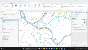
This chapter focuses on vector spatial analysis and geoprocessing tools used to answer geographic questions and solve spatial problems. Geoprocessing allows GIS users to combine datasets, run spatial operations, extract target areas, and build automated analysis workflows. The chapter introduces core vector processing tools including buffering, clipping, intersecting, unioning, erasing, and querying features by attributes or spatial locations. By overlaying multiple vector layers such as land use zoning, flood plains, demographic boundaries, and transportation corridors. GIS analysts can evaluate land suitability and measure environmental impacts.
Tutorial: this chapter shows how to:
- Vector spatial analysis tools
- Create single and multiple-ring buffers around features
- Clip feature layers using spatial boundary polygons
- Intersect spatial layers to identify overlapping areas
- Union feature classes to combine geometric structures and attributes
- Erase unwanted spatial features from analysis boundaries
- Execute attribute and location queries
- Select features by attributes using SQL expressions
- Select features by location using spatial relationship rules
- Combine attribute and spatial selections for refined analysis
- Automate geoprocessing workflows
- Open and navigate Model Builder
- Add tools, datasets, and connectors to a Model Builder canvas
- Set model parameters and run automated spatial models
- Export models to Python scripts or share as geoprocessing tools
This chapter was very interesting as it showed how spatial overlay tools and Model Builder work together to automate repetitive geoprocessing workflows and analyze geographic relationships without manual repetition.
Chapter 10:
This chapter covers raster GIS and surface analysis techniques used to study continuous spatial data. Unlike vector data which uses points, lines, and polygons for discrete features, raster data represents continuous geographic phenomena with the use of a regular grid of square cells where each cell holds a specific numerical value such as elevation, rainfall, temperature, or land cover type. The chapter explains the display and reclassification of raster grid layers, derivitization of continuous terrain surfaces from Digital Elevation Models (DEMs), performance of map algebra calculations, and creation of suitability models to evaluate prospective locations for developments or conservation projects.
Tutorial: this chapter shows how to:
- Work with raster datasets and elevation models
- Display and symbolize single-band and multi-band raster layers
- Derive surface maps: Hillshade, Slope, Aspect, and Contour
- Perform raster analysis and map algebra
- Reclassify raster cell values into standardized numeric scales
- Use the Raster Calculator for map algebra expressions
- Calculate Euclidean distance rasters from target features
- Conduct suitability modeling
- Combine weighted suitability rasters to identify optimal locations
- Execute Zonal Statistics as Table to summarize raster values within vector boundaries
I learned a lot in this chapter about raster processing, surface modeling, and how map algebra can be used to solve spatial suitability problems.
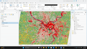
Chapter 11:
This chapter introduces 3D GIS visualization and lidar point cloud analysis. 3D GIS expands traditional 2D map analysis by incorporating height and elevation values (Z values), allowing users to view, measure, and analyze realistic 3D building structures, urban landscapes, terrain models, and spatial visibility. Lidar (Light Detection and Ranging) technology uses laser sensors mounted on aircraft or terrestrial scanners to collect dense point clouds containing millions of 3D points that represent ground surfaces, vegetation canopy heights, and building structures. The chapter covers converting 2D maps into 3D scenes, filtering and displaying LAS point cloud datasets, extruding 2D building footprints into 3D models, and executing spatial visibility analysis.
Tutorial: for this chapter, it shows how to:
- Navigate and create 3D scenes
- Convert 2D maps into 3D Local and Global Scenes
- Navigate 3D scene environments using camera controls and elevation surfaces
- Work with lidar and LAS datasets
- Add LAS point cloud datasets to a 3D scene
- Filter LAS datasets by elevation, return intensity, and classification codes
- Create Digital Elevation Models (DEM) and Digital Surface Models (DSM) from LAS datasets
- Build 3D urban features and spatial analysis
- Extrude 2D building polygons using height attribute fields
- Apply multipatch 3D symbology and textures to building models
- Conduct Line of Sight and Viewshed analysis in 3D space
This chapter was very interesting in showing another way to visually display the data using 3D scenes