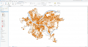
GIS Tutorial Chapter 7:
Chapter 7 of the GIS tutorials was about digitizing. The first tutorial involved editing features to move a building’s polygon. This is done by using the move tool and clicking the select button, then clicking on the building bookmark that they provided. Following this, you rotate the features next as well as add more vertex points and split features. This tutorial was exceptionally challenging while dealing with the polygon editing because of how stubborn the tool could be when trying to adjust the shape. Tutorial 2 was similar but involved creating a polygon feature class and fields using the Create Feature Class tool and applying the given settings. Following this, you utilize the trace tool to outline an entire area rather than a particular building. Tutorial 3 was the easiest of this chapter because all you had to do for this tutorial was use the smooth polygon tool and apply the settings that they provided and click run. The final tutorial, tutorial 4, uses the coreference tool to adjust the CAD drawing and then export the file. The georeference tool allows you to adjust the group and add control points. These control points give the ability for the CAD drawing to be highlighted and form a rough shape of the designated building. You finish this tutorial by exporting the file and then classifying the layers, which display the spaces of each room more accurately. To finish this tutorial and this chapter, you simply click the transform button found within the modified features pane to move the drawing to its precise location.
Screenshots: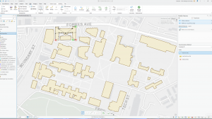
GIS Tutorial Chapter 8:
Chapter 7 is about geocoding and only has 2 tutorials; however, it is still complicated and was one of the more challenging chapters so far. The first tutorial was about geocoding using zip codes. This tutorial began by using the create locator tool and inputting the settings that the textbook provides. You can then view this locator after clicking run within the locator tab. In order to actually geocode the data by zip codes, you must next click the geocode addresses tool and once again apply the various settings. After changing the symbology for the new layer, you can view the individual mark for each zip code centroid. You must then rematch attendee data by zip code by right-clicking attendees, data, and rematch addresses. You then input the number 15213 and click the match button. To finish this tutorial, you open the collect events tool, apply the given settings, and click apply to count the zip codes and apply graduated symbols for the given marks. The next tutorial, tutorial 2, is similar to the previous tutorial however, this tutorial is about geocoding with street addresses rather than zip codes. Once again, you first open the collect events tool and apply the necessary settings, and run the tool. You then open the geocode addresses tool, apply the settings, and click run. For this one tutorial, you must select the minimum candidate and matching scores and finally produce the final results and view the map.
Screenshots: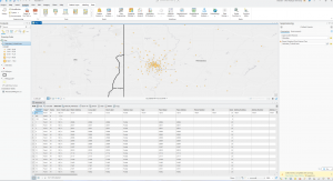
GIS Tutorial Chapter 9:
This is the final required chapter for this course’s discussions and was surprisingly easy compared to previous chapters. The first tutorial used the pair-wise buffer tool and inputted the given settings to estimate individuals who live in close proximity to the nearest pool. You then click select by location and apply the settings and click summarize to finish the first tutorial. The next tutorial is very simple and involves adding a buffer ring around the same map points as the previous tutorial. You can simply search for the multiple ring buffer tool, apply the settings, and then use the spatial join tool to join attributes and summarise data inside the ring. The next tutorial was the most challenging of this chapter for me, but was still straightforward. The first step of this tutorial was to create multiple-ring service-area polygons. The select by attributes tool does this: applying the settings, clicking the service area layer, clicking input data, clicking import facilities, and applying all the settings. The next step is to join service areas and pool tags by spatially using the spatial join tools and selecting pooltags. After this step you must calculate pool use for statistical areas within the attributes table, then make a scatterplot in the features layers data tab in the visualize group, and finally fitting a curve to the data points by opening the chapter 9 data and inputting data for Beta. The next tutorial is using Network Analyst to locate facilities. You must go into the input data group, click import facilities, and apply the settings, then import demand points and apply the settings, then adjust the types and run the mode. You must then analyze the optimal solution for this by opening the various attribute tables and using the summarize tool. The final tutorial is forming data cluster analysis which is done by using the Multivariate Clustering tool, applying the settings, and interpreting the clusters by adjusting the clusters in the label column.
Screenshots: