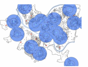
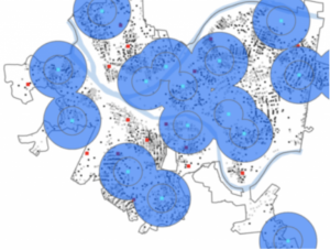
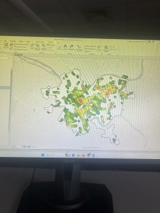
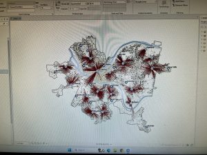
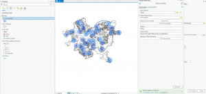
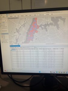
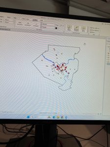
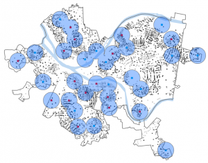
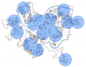
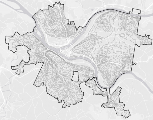
Chapter 9 went into “Spatial Analysis”. We started with buffers, which are basically zones around features. You set a distance (like, say, a half-mile radius around all the schools), and ArcGIS draws a polygon. It’s useful for seeing what’s “nearby.” I played around with creating buffers around pools in Pittsburgh, which was a case study that was built on throughout the chapter, to see how many kids lived within a reasonable distance. Then we got into multiple-ring buffers, which are like bullseyes – multiple buffers at different distances, all around the same feature. This allows you to see, for instance, not just who’s within a mile, but who’s within a half-mile, a quarter-mile, and so on. You can get pretty granular with it. The part that got my head spinning a bit was service areas. These are like buffers, but instead of straight-line distance, they measure distance along a network, like roads. This makes way more sense for real-world situations! If you want to know how long it really takes to get somewhere, you need to consider streets, not just draw a circle on a map. I found myself getting a little lost during the section on setting the parameters. The last thing the chapter covered was cluster analysis, which is finding patterns in data points. The example was looking at crime data and trying to find clusters of, say, crimes committed by a certain age group, or a certain type of crime.
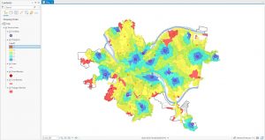
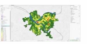
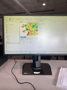
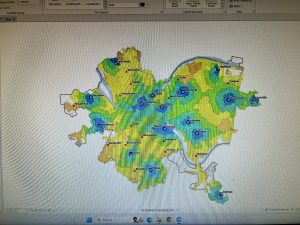
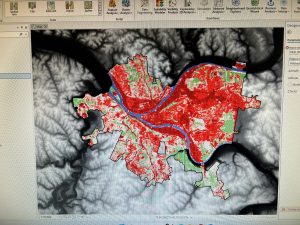
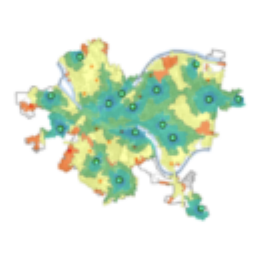
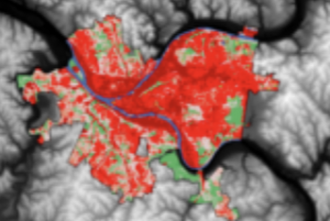
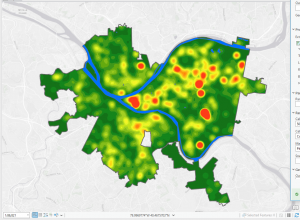
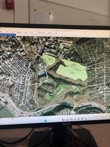
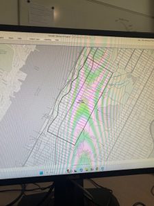
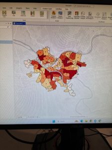
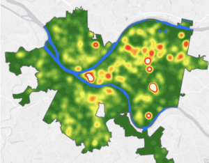
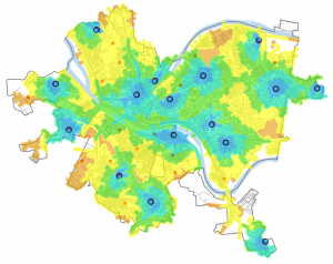
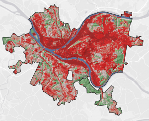
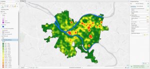
Chapter 10 was a shift from the previous ones because it focused on raster data, not vector data. Each pixel has a value, and that value can represent all sorts of things – elevation, land use, temperature, you name it. We started by exploring some existing raster datasets, like elevation data for Pittsburgh. The “hillshade” tool was particularly cool; it’s like shining a virtual light on the elevation data to create a 3D effect to help visualize the terrain. Next, we looked at kernel density maps. It was interesting to see how we could estimate and visualize that distribution using the kernel density tool. A big part of the chapter was about building a model. This was a new concept for me. Basically, you’re creating a set of instructions for ArcGIS to follow, step-by-step. The example was building a “poverty index” by combining different raster layers, like population density and income levels. I got a little confused with the “in-line variable substitution” part, where you use variables to represent values in your model. The chapter wrapped up with running the model and seeing the results, which was pretty satisfying!
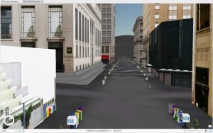
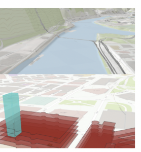
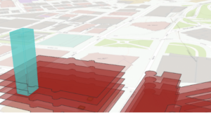
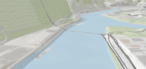
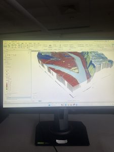
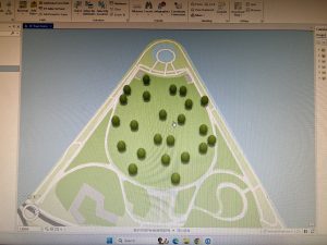
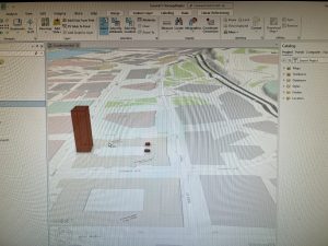
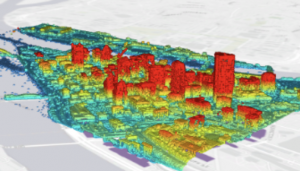
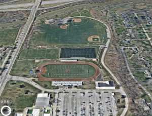
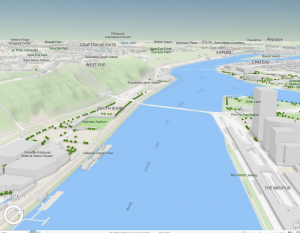
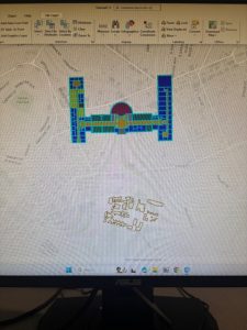
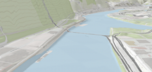
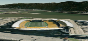
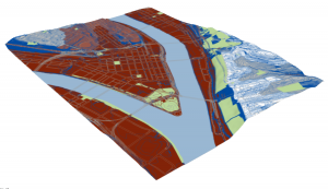
Chapter 11 was visually the most exciting! It’s all about working with data in three dimensions, which opens up a whole new way of looking at things. We started by exploring a global scene of Pittsburgh, which uses the earth’s curvature. I learned how to navigate around (pan, zoom, tilt) using the mouse and keyboard shortcuts. Then we switched to a local scene, which is better for smaller areas where the earth’s curvature isn’t as important. We created a TIN surface, which is a way of representing terrain using triangles. It’s like connecting a bunch of points with lines to create a 3D model of the ground. The book reads that you can use it to create the surface on which features like buildings will be rendered. The coolest part was working with lidar data. Lidar is like radar, but with lasers, and it creates incredibly detailed 3D point clouds. We used it to visualize buildings and even to estimate the height of a bridge, measuring the distance between the top and bottom of the bridge’s span. We also looked at procedural rules to make 3D buildings automatically. You can set parameters like building height and roof type, and the software generates the building for you. This seems like it would be incredibly useful for creating large-scale city models. I did run into an issue where I was using the incorrect view, but I think I got that sorted out. At the end, I made an animation, which was a fun way to end the chapter. It’s like creating a fly-through of your 3D scene. I’m still a bit confused about all the different options for exporting the animation, but I managed to create a basic movie.