Week 6
Chapter 7
This chapter puts to practice how we draw polygons and define areas using the GIS. Most of our work for this chapter was spent defining areas using polygons and manipulating those polygons to fit the buildings present on the CMU campus. I think it is interesting that they used Carnegie Mellon because I feel like I remember reading something about them having some sort of tie to GIS work.
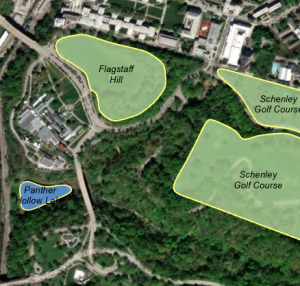
One of the most fun parts of this chapter and consequently probably the easiest was smoothing polygons to fit real vectors. We did this for several golf course greens and a small lake.
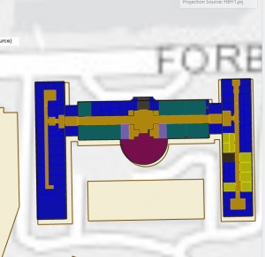
This second picture is the image of a CAD drawing I input into the GIS. It took me forever to find it and I was worried I had messed something up but then I zoomed to the layer and found it in Cincinnati.
Chapter 8
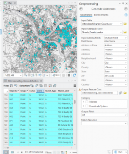
Chapter 8 put focus on geocoding which is the geographic signature attributed to different points. We first worked to correct some database values that needed some correcting in a registry of attendee addresses. We also did some fairly basic display changes. In the second part we worked on matching address fields with the address we are given to the correct address table. We also checked for the accuracy of each of the matches and the overall successful match count.
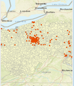
Above is a map of all of the addresses in the attendee address database.
After matching the data in the attribute table we ran a select by attribute based off of the accuracy score of the address matching(score 90 or above). Those fields were highlighted and then the map updated to show the addresses we had a match on vs. the ones we don’t have a match for.
Chapter 9
Chapter 9 focused on spatial analysis and drawing boundaries around distance to points. This chapter’s work was focused in the city of Pittsburgh where the analysis was on pool availability for the youth and in the last module crime. I found this module to be pretty challenging at times but mostly that was because I was not reading the directions thoroughly and looking for the right buttons. The first two modules introduced buffer rings to show locations around a point and how to add multiple of these buffers around one single point.
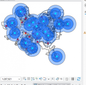 We then created a map called a gravity model which instead of showing distance to a point as equidistant use more complex real world logic to discover the distance to the nearest pool(pictured below)
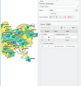
We also created a spider plot graph to show distances without a set color interval. Each of the lines connects from a pool to a block centroid. Finally we organized crime data to come to spatial conclusions about different demographic groups and their crime impacts.