Chapter 4:
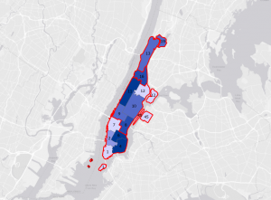
This chapter covers spatial and regular databases. Using the .gdb extension, which is not a file extension but merely a folder. The first section starts us off by importing data into a project. Next using the capabilities of a database in the Catalog pane. This allows us to alter or copy geodatabases. The chapter mentions the importance of columns in data tables, where most attributes are handled. 4-2 discusses modifying attribute tables, using the calculate field tool (I found this part a bit confusing but later figured it out), and joining/exporting features. The same section also shows how to calculate fields and draw out/concatenate (basically combine; e.g., “Bob” + “Bob” = “BobBob”) string fields. The section after I thought was the most interesting, where we connect data from tables to feature classes. This is done with SQL queries regarding filtering, which contain 3 parts: the attribute name, a logical operator (<, >, etc.), and an attribute value. (Haven’t heard of SQL since my Intro to Database Fundamentals class a good minute ago.) There are 2 types of queries: simple and complex. Simple queries use 1 connector, while complex queries use 2 or more. Connected by the operators an and, or, an or. Queries can be used to filter out features based on certain characteristics like age, time, (in this chapter) type of crime, and location. Section 4-4 was a short section on how to aggregate data with spatial points. Later, the chapter showed us how to use central points for shapes. I thought of this as basically adding a dot, where the dots represent the number of burglaries by neighborhood. The last section of the chapter had us create a new table to help the user simplify data by reducing duplicates. Overall, I thought this chapter was pretty interesting to work with.
Chapter 5:
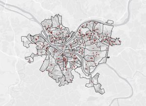
In the last chapter, we learned about filing geodatabases; in this current one, we learn more about spatial databases specifically. In the first section, we used coordinates and changed world map projections. I think I spent maybe 20-30 minutes looking at all the types of projections that the GDB file had to offer. The next section had us working within the subject, but within the U.S. Not only that, but the chapter also discusses how to set reference zones to help select projected coordinates. Based on what area the user wants to study. One of the most interesting things I learned from this chapter was how to add new layers on a coordinate system. Later, we changed the map coordinate system; this process was pretty easy. I originally thought it would be harder than that, or at least more complex. The following section has us working with vector data formats. This required importing a shapefile, adding x and y coordinate data, and finally converting a KML (Keyhole Markup Language) file into a feature class. 5-5 really gets into real-life data through the U.S. Census, requiring us to download specific data sets. I never even knew a website like that could exist. I also spent some time going through the website, checking the menus and data from other cities. After all this information was downloaded, it was entered into GIS. This section took the longest because I messed up a step along the way and had to repeat the process. When all the information is gathered, the collected data is joined and turned into a choropleth map. Learning how to download geospatial data was pretty straightforward, as was adding it to the current map. When this chapter was finished I explored some agency maps, this specific chapter piqued my curiosity.
Chapter 6:
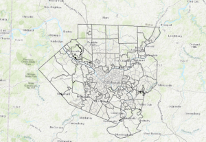
In the previous chapter, we learned to search through geographic databases, either by collecting the information ourselves or through another source, like a government agency. The sixth chapter focuses heavily on geoprocessing and its use cases to build our areas of study. The first section of this chapter had us delete features to create new ones using the Pairwise Dissolve function. This totals the attributes using statistics like count, sum, and mean. Next, we clip (a geoprocessing tool) and extract those features for the purpose of studying them. By using Select By Attribute (this part was easy) and the Select function, a bit annoying to use because I couldn’t figure out how to use it correctly. After that, we combined water features using the merge function. This tool basically combines two or more feature classes into one. Then we used the Append tool to add data from one source to another dataset. (Haven’t heard this word since my Python Class maybe a year or two ago.) Next, we intersected those features to determine their specific zones. This part of the chapter uses the Pairwise Function once again but with a new tool called Intersect. This new tool removes any input layers that do not overlap. Then we use a tool called Union to overlay the attributes and space of specific layers to create a new one. Finally, the chapter closes out with us using the Tabulate Intersection. The results show us the calculations of how map layers overlap, which it outputs in the table. Overall, I thought this chapter was a bit complex, but I learned a lot from this part of the book. The complexity comes from performing a bunch of new tasks with newer functions. As well as learning what these new functions specifically do and their uses.