Redman Week 5

Part Two: Preparing Spatial Data for Use

Chapter 4: File Geodatabases 

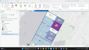
In this chapter, the focus changes from the visual aspect of maps to the data behind it. Chapter 4 shifts from map layouts to managing spatial data in the file Geodatabase, which is ESRI’s storage system. File geodatabases serve as organized storage for feature classes, raster datasets, and attribute tables. This is useful in research, spatial analysis, and keeping records. The purpose of this chapter is to learn how to organize project data, import external shapefiles and tabular data into a project geodatabase, modify field attributes, and execute relational joins and spatial queries in ArcGIS Pro.

Terminology:

• File geodatabase (.gdb): ESRI’s database used to store feature classes, raster datasets, and standalone attribute tables optimized for ArcGIS Pro.
• Feature class: A collection of geographic features with the same geometry type (point, line, or polygon) and identical attribute fields stored in a geodatabase.
• Shapefile: A legacy vector data storage format for storing the location, shape, and attributes of geographic features, commonly converted into feature classes for geodatabase use.
• Table join: An operation that appends the fields of one table to another based on a common matching attribute field across both datasets.

Tutorial: The tutorial was very helpful in learning how to navigate spatial data management. It showed how to:

• Import data into a new ArcGIS Pro project
  • Create an ArcGIS Pro project
  • Set up a folder connection
  • Convert a shapefile to a feature class
  • Import a data table into a file geodatabase
  • Use database utilities in the Catalog pane
• Modify attribute tables
  • Delete unneeded columns
  • Add a field and populate it using the Calculate Field tool
  • Join a data table to a feature class attribute table
  • Export a feature class to make a join permanent
  • Calculate the sum of fields
  • Calculate the percentage of total population under 20 years old
  • Extract substring fields and concatenate string fields
• Carrying out attribute queries
  • View crime incidents
  • Create a date-range selection query
  • Reuse a saved query to create a definition query
  • Query a subset of crime types using OR connectors and parentheses
  • Query the day-of-week range
  • Query person attributes
• Aggregate data with spatial joins
  • Build a spatial join
• Use central point features for polygons
  • Create a central point feature class for polygons
  • Create a point layer
• Create a new table for a one-to-many join
  • Create a table
  • Make a one-to-many join

Overall, I learned a lot in this chapter about backend data management. Cleaning up attribute fields and setting up relational joins makes spatial analysis more organized and increases efficiency

Chapter 5: Spatial data

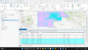
This chapter focuses on spatial data formats and coordinate systems used for mapping locations accurately on Earth’s surface. It explains geographic coordinate systems, world map projections, US map projections, and setting projected coordinate systems for local, state, and national maps. The chapter also demonstrates how to work with vector data formats, download spatial and tabular data from the US Census Bureau, and source ready-to-use geospatial datasets from external repositories.

Terminology:

• Geographic Coordinate System (GCS): Three dimensional reference system that uses latitude and longitude angular units (degrees) to measure locations on the Earth’s surface.
• Projected Coordinate System (PCS):  Two dimensional planar surface that uses a mathematical transformation to project the Earth’s spherical surface onto a flat map.
• State Plane Coordinate System: A set of 126 geographic zones dividing the United States to provide localized, high-accuracy projected coordinate systems with minimal distortion for local government and surveying work.
• Geospatial data: Digital spatial data that represents geographic features and can be rendered into vector layers, raster datasets, or web services in GIS software.

Tutorial: For this chapter, the tutorial shows how to:

• Examine world map projections
  • Examine distortions in latitude/longitude maps
  • Apply world projections like Hammer-Aitoff and Robinson on the fly
• Change map projections for national maps
  • Change map projections to Albers Equal Area Conic
• Set local coordinate systems
  • Look up State Plane zones in ArcGIS Living Atlas
  • Apply localized coordinate systems and project geographic layers on the fly
  • Configure map display units to feet or meters
• Work with vector data formats
  • Convert shapefiles into file geodatabase feature classes
  • Plot point layers from XY coordinates
  • Convert KML files to feature classes using KML To Layer
• Download Census Bureau spatial and tabular data
  • Download TIGER shapefiles and demographic data from the US Census Bureau
  • Join demographic tables to spatial boundary layers using GEOIDs

I learned a lot in this chapter about coordinate systems and projections. It was very helpful to see how changing projections prevents spatial distortion when analyzing geographic areas.

Chapter 6:Geoprocessing

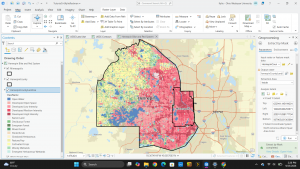
This chapter covers geoprocessing tools and workflows used to extract, aggregate, overlay, and analyze spatial features. Geoprocessing is used as a tool in ArcGIS Pro to isolate specific geographic study areas, combine overlapping dataset boundaries, and apportion demographic attributes in unaligned spatial units. In this chapter, the text shows how to process and prepare layers for emergency management officials in Manhattan and the Upper West Side neighborhood.

Terminology:

• Geoprocessing: A fundamental GIS framework and set of analytical tools used to manipulate, process, extract, transform, and evaluate spatial data to perform spatial analysis.
• Pairwise Dissolve: Aggregation tool used to remove interior polygon boundaries sharing a common attribute while calculating summary statistics across combined shapes.
• Pairwise Clip: An extraction tool that acts as a boundary cutter, keeping only the intersecting portions of input features within a specified boundary polygon.
• Apportioning data: A method of estimating tabular attributes for custom target zones by calculating the proportion of spatial overlap between non-aligned polygon boundaries.

Tutorial: This chapter shows how to:

• Dissolve features to create higher-level boundaries
  • Open attribute tables for block groups and examine housing attributes
  • Run Pairwise Dissolve on block groups to remove interior boundary lines and sum housing units by neighborhood
  • Dissolve fire companies to create fire battalion and fire division feature classes with population totals
• Extract features for a study area
  • Use Select By Attributes to isolate a neighborhood boundary and export it as a study area
  • Use Select By Location to extract block groups and street segments intersecting the study area
  • Execute Pairwise Clip to trim street networks cleanly along perimeter boundaries
• Overlaying datasets
  • Merge separate borough water feature layers into a single consolidated water dataset
  • Append firehouses and police stations to an existing EMS facilities point layer
  • Intersect streets and fire companies using Pairwise Intersect to assign response responsibilities
  • Run Union on neighborhood and land-use layers to calculate land-use areas
  • Use Tabulate Intersection to apportion demographic population data between census tracts and fire zones

This chapter was helpful in teaching about how spatial overlay tools work together to aid in urban planning and emergency management tasks.