Mitchell, Chp. 4
Chapter four described mapping density, which is symbols on a map marking the density of a given set of data. The purpose of this is to highlight where the highest or lowest density of the targeted set of data is. An example of this could be a construction crew viewing a city map with red dots marking every pothole within the city’s sidewalks and streets. Utilizing GIS mapping to view where the highest density of potholes in the area are, the construction crew could make the choice of where their next road replacement should be based on deductive reasoning. This example demonstrates how mapping density of a data variable can be utilized for tracking disease, weather patterns, public transportation, etc. This form of data display has infinite uses and is extremely simple and self explainable. Learning about the various cells and calculations needed for situations requiring density values surprised me. These calculations are crucial because there are several parameters that can affect how the GIS calculates the density surfaces. The factors that affect the GIS calculations are: cell size, which determines how coarse or smooth the patterns in the GIS map will be. In order to have a smooth surface, you must create more and smaller cells, which in turn demands more on your computer, like processing and storage space, which slows down the processing time for making the map. A coarser map looks rougher because of the larger cells however, with bigger and fewer cells the less strain on your computer while processing. Search radius is the maximum distance setting of a data point, which also affects the GIS system similarly to cell size. The larger the search radius, the more generic the patterns are, and the smaller the more detailed. The calculation method uses two different methods to determine cell size. The simpler method only calculates the features within the search radius of a data cell, whereas the more complex method uses a mathematical function to expand on complex features closer to the center of the cell, not just within the search radius. The last factor that affects the GIS calculations is units, which is the unit of measurement required for the mapping density of the GIS map. These factors all play crucial roles for the desired accuracy required for each map.
Mitchell, Chp. 5
The next chapter, chapter five, describes mapping what is inside a given area. This can be done to monitor what may be happening in an area, prepare for a predicted outcome, analyze data within an area, and more. In order to find out what’s inside a set area, a boundary line is drawn and data points within the area are displayed. In Andy Mitchell’s textbook (chp.5) they show the following image: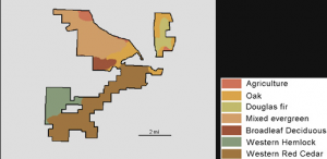
Andy Mitchell, 2020, pg. 144) This image demonstrates GIS mapping what tree species are inside a selected area in order to view where certain tree species prefer. This image helped me understand what this chapter of the book was described by displaying a real world example of how this information could be used such as a log company looking for specific tree species, a conservation group looking for native and diverse wooded habitat and tree species, a township looking for water patterns in the area based on which trees prefer which area, and etc. In order to actually determine what is inside, there are three ways of finding it out. The three ways are drawing areas and features, selecting the features inside the area, and overlapping the areas and features. Drawing areas and fields is good for finding out if features are inside or outside an area however is quick and easy for visuals but lacks information about the inside features. Selecting the features inside the area is good for getting a list or summary of features inside an area however, it does not tell you what is inside each of several areas. The last method, overlapping the areas and features, is good at finding out which features are inside which areas and summarizing how many or how much by area, however, it requires a significant amount more processing and strain on your computer. In summary, these methods have their strengths and weaknesses, and each is used for separate features and utilizations.
Mitchell, Chp. 6
Chapter five discussed mapping inside an area, chapter 6, however, discusses mapping finding what is nearby an area. Finding what is nearby can be crucial for finding out what is happening in a given distance and finding out what is within traveling range. There are two measurements in GIS when it comes to measuring distance: one is distance, and one is cost. Distance is obviously how far from point A to B, but cost is how much time it would cost. An example of cost over distance might be the national park rescue service that may only have to hike 4 miles to get to someone, but they have a high time cost of climbing over the mountain and across the river. Time is money and is one the biggest expenses, so measuring the time commitment aids in accurately reflecting in the GIS mapping. The three ways of finding out what’s nearby is straight-line distance, distance or cost over a network, and cost over a surface. Straight-line distance is exactly how far from point A to B in a straight line and is good at setting a boundary and measuring the distance of one point to another. Distance or cost over a network accounts for linear features and adds a cost of time besides distance, and is good for finding what is within travel distance as well as cost. The final method, cost over a surface, specifies the location and travel cost, and people primarily utilize it for over-landing off primary roads. These methods all have their own uses, and not one fits all. They each are utilized in various situations, such as when I gave an example of the NP rescue service they would use cost over surface. Furthermore, users frequently add buffers and boundaries to create a zone around given features. This addition helps measure cost and distance, ensuring an accurate measurement.