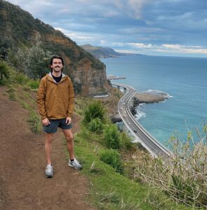
Hi! My name is Jonathan Munroe and I’m a junior from St. Louis, Missouri. I’m majoring in geography with a minor in music performance (violin). I’ve taken quite a few classes regarding GIS but I’m excited to take this course specifically on ArcMap. After graduation I’d either like to work for a nonprofit urban planning agency doing neighborhood revitalization without displacement or work making maps out in the woods for the forest or national park service.
Schuurman Chapter 1- Introduction to GIS: I found this passage very interesting, as I’ve read about the history of map-making and remote sensing but I’ve never learned about the history of GIS. The program itself is so versatile and especially in today’s age, it’s widely popular and sought after. As an example, last year when I worked at the Flying Pig I was talking about my major to a customer who worked for Nationwide in Columbus. He told me that if I got a degree or certificate in GIS I should come to him and he’d have a job ready for me. While insurance isn’t a field I’m interested in, I think the story speaks volume and adds on to Schuurmans emphasis on how popular GIS has become in recent years. Another thing I found fascinating was his topic of visualization where he said “visualization is used to manufacture meaning from data…people are able to discern information from visual display with greater facility than from tables or printed text.” I’m a visual learner myself and think my love for maps stems from my availability to understand the data. Schuurman further proves his point by saying that “people ‘reason’ using imagery. GIS can better connect, market and convey any information, which is why it’s so sought after in the job market. This reading has made me excited to take this class through the semester and become more knowledgeable and familiar with GIS, helping me excel my research skills, resume and general knowledge.
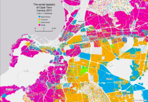
For my map, I chose to look at the racial segregation of Cape Town, South Africa with the failure of the Group Areas Act of Apartheid. I chose this map because I’m currently writing a TPG to visit Cape Town regarding racial housing segregation in comparison to the Red Line Policy of the United States. This map shows the racial composite of Cape Town using census data from 2011.