Making New Shape Files from Existing Shapefiles
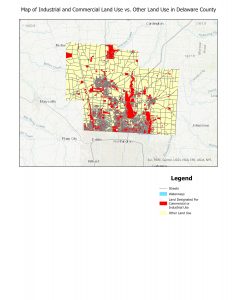
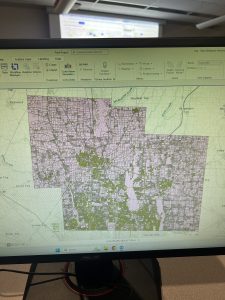
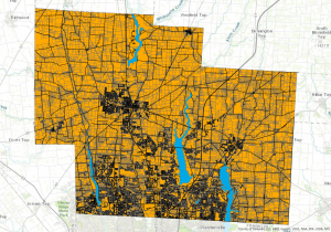
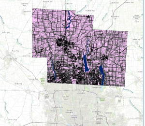
The first application I chose to execute on this final was to find two related datasets within the pre existing dataset, and export them into a separate map. To do this, I first put the hydrology, Street Centerlines, and the parcel data set shapefiles for Delaware County into my new project in ArcGIS Pro. Then, I decided that I wanted to isolate the land used for commercial and industrial purposes because this land is privatized and non-residential, which means they are very similar land uses that can be combined in a map to better understand the land use of the county. I thought this map could be useful for residents and experts when looking at the zoning of the county and where the commercial and industrial lands are located.
In order to create this map I had to create a separate shapefile for this layer of the combined industrial and commercial land in the county. To accomplish this, I had to first open the attribute table of the parcel layer. Then, I chose select by attributes, and chose the data points–polygons–that had a class number beginning with 3 (for industrial uses) or 4 (for commercial uses). After that, I had to right click the layer in the contents pane and choose data, then export selected data. This created an export shapefile that I was able to put into a map over top of the other parcel layer and added the hydrology and street centerlines layers to provide the context for the rest of this map. Specifically the streetlines are helpful for this because you can see what the transportation around all of the properties zoned for industrial and commercial use is like, and how the land use compares to the density of the streets.
I then created a new layout, put in this map, and zoomed to the most recent active map view. I manipulated the symbology of the layers to be most readable and to have good contrast. Next, I continued to spruce up the presentation of the map by changing the layer names to more presentable versions of their meanings, and adding a legend of the symbology I used on each layer. Finally, I added my title and exported the layout as a jpeg.
Mapping Change

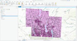
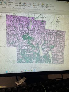
The second application I chose for the knowledge of ArcGIS Pro I gained during this course was mapping the change of subdivisions in Delaware County since the beginning of its settlement in the 1800s. First I imported the shapefiles for the street centerlines, hydrology, and subdivisions data sets. Then I changed the symbology of the subdivisions layer to graduated colors. I had to organize it by the field: REC_DATE, which was the date of the construction of those subdivisions in the form YYYYMMDD. I set the upper bound of each section to the first day of the year for the corresponding year, and noticed that no subdivisions were from before 1800. Then I changed the colors of the symbology to be easily distinguishable. Next, I removed all the outlines of these polygons to allow for easy viewability from the larger frame of the map. Finally, I created a layout and took all the same steps as with the first map to make the layout presentable and understandable for the reader.
