Author: logdog

Delaware Data Info:

Zip Code: All the zip code areas for Delaware County. Updated regularly/as needed

Recorded Document: shows the places where recorded documents such as plat books are located (books that show how the county property is divided/landlines). other info on data collected on these lands such as annexes, surveys, etc. is also stored and represented by the dots for where they are kept.

School District:  All the school districts within Delaware County.

Map Sheet: all map sheets in Delaware County.

Farm Lot: Map of all the farm lots in Delaware County provided by the US military and Virginia Military Survey Districts.

Townships: Shows the 19 townships in Delaware County,

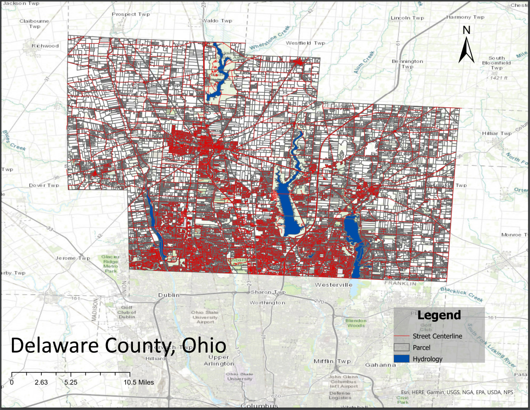
Street Centerline (data)/ Street Centerline – DXF (document): All documented private and public roads in Delaware County. Put together using observational data, regularly updated/as needed.

Annexation: Delaware Counties’ annexed land and growing boundaries from 1853 to the present. Annexed land means land that was taken into the city limits.

Condo: All recorded condominium polygons in Delaware County.

Subdivision: All subdivisions and condos in Delaware County.

Survey: Shapefile of all survey points taken in Delaware County, excluding old surveys in volumes 1-11. All are certified surveys and more after 2004 are being added regularly.

Dedicated Row:  All road right-of-ways ROW owned by the city. These are the areas of grass/sidewalk on the side of a road that is owned by the city. Not all roads have one.

Tax District: All tax districts in Delaware County.

GPS: All GPS monuments from 91-97. Uses Universal Mercator Northing and Easting.

Original Township: Original township and boundaries before tax districts changed shape.

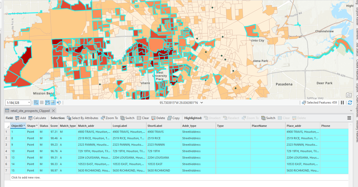
Address Points (data)/ Address Points– DXF (document): Point layer of all address points in Delaware. Intended to support appraisal mapping, 911 Emergency Response, accident reporting, geocoding, and disaster management. The layer provides the capability to reverse geocode a set of coordinates to determine the closest valid address.

Precinct: Voting precincts in Delaware County.

Hydrology: All major waterways in Delaware County.

Building Outline 2021 (data)/ Building Outlines – DXF (document): All building/structure outlines as of 2021.

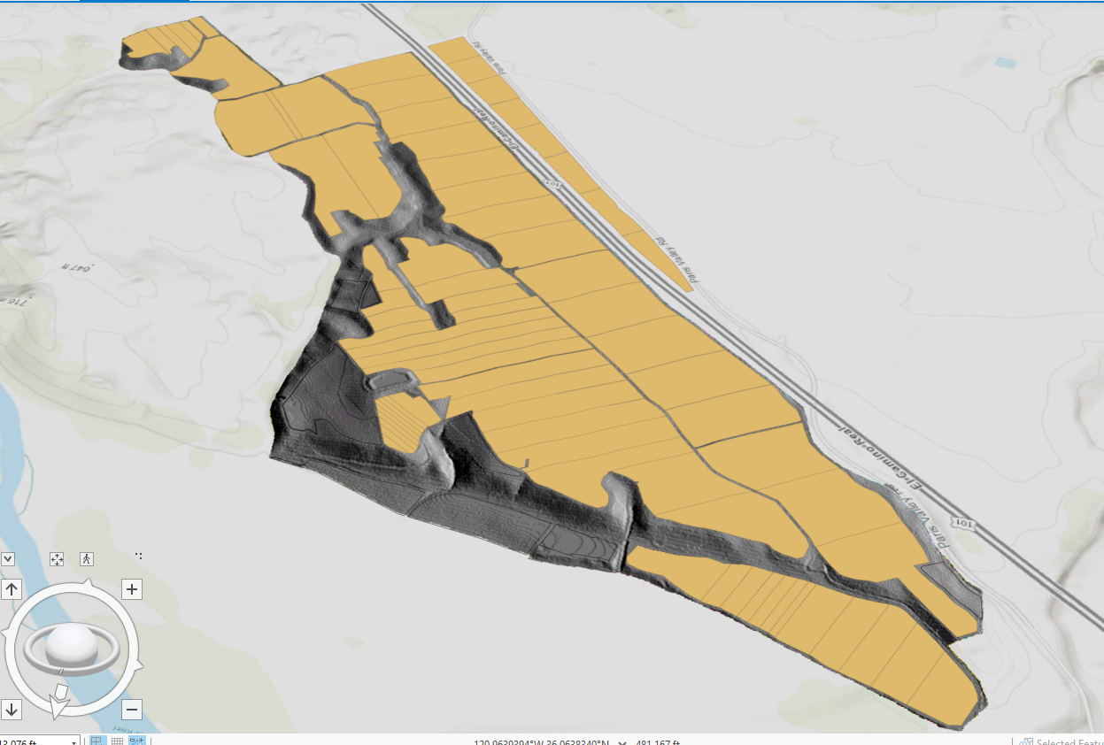
Parcel: Cadastral Parcel lines in Delaware County (property lines for real estate). Also holds appraisal information.

PLSS:  created to facilitate identifying all of the PLSS and their boundaries in both the US Military and Virginia Military Survey Districts of Delaware County. PLSS is a survey system made in 1785 to establish parcel lines with a standard system.

2022 leaf-On Imagery (SID) (Map): 2022 Imaergey 12in Resolution map. A SID file is a compressed file of GIS data.

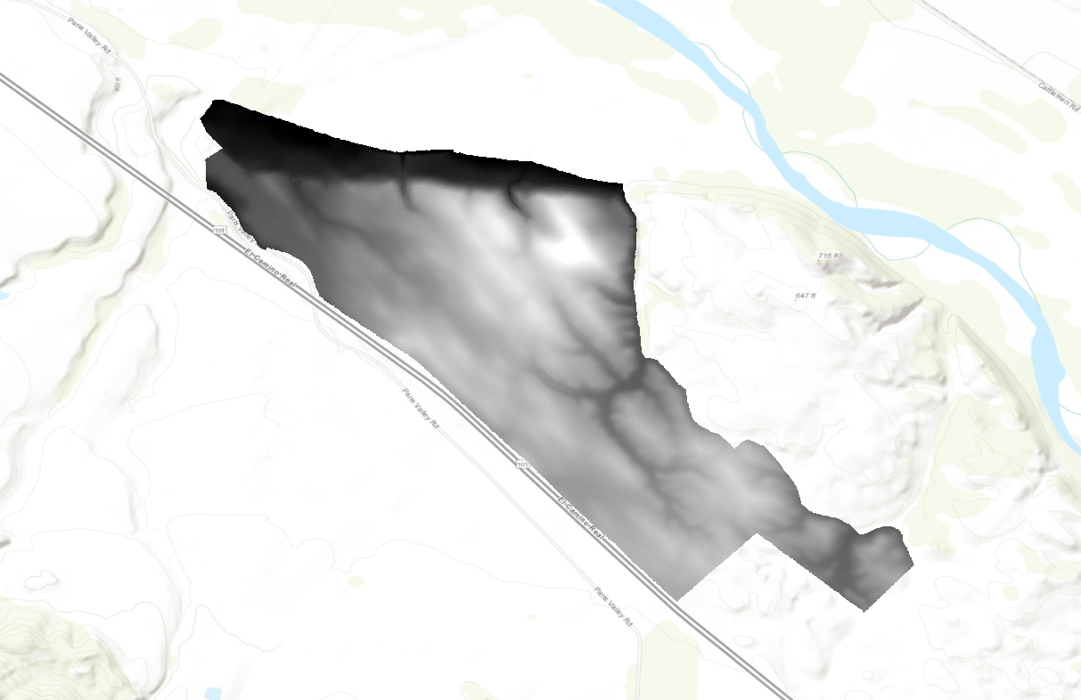
Delaware County Contours: 2ft contours of Delaware County from 2018.

2021 Imagery (SID File) (Map): just saw “Delaware County Ohio”.

Delaware County E911 Data: all certified addresses in Delaware County. Provides the capability to reverse geocode a set of coordinates to determine the closest valid address and is intended to provide 911 agencies with the information needed to comply with Phase II 911 requirements.

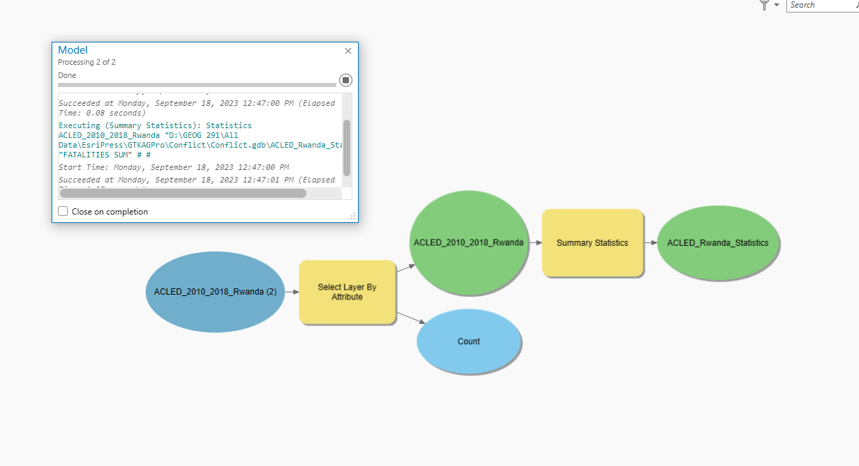
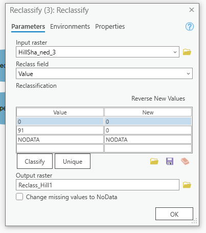
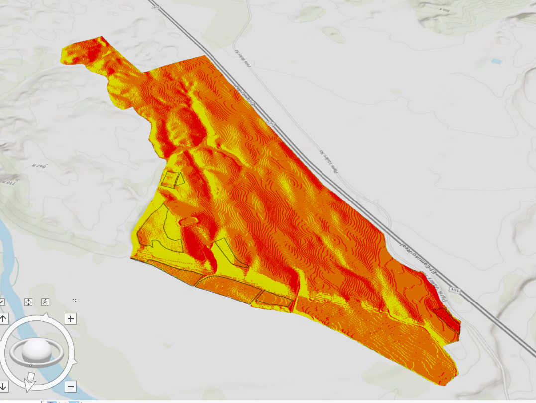
ArcGIS Pro Portion:

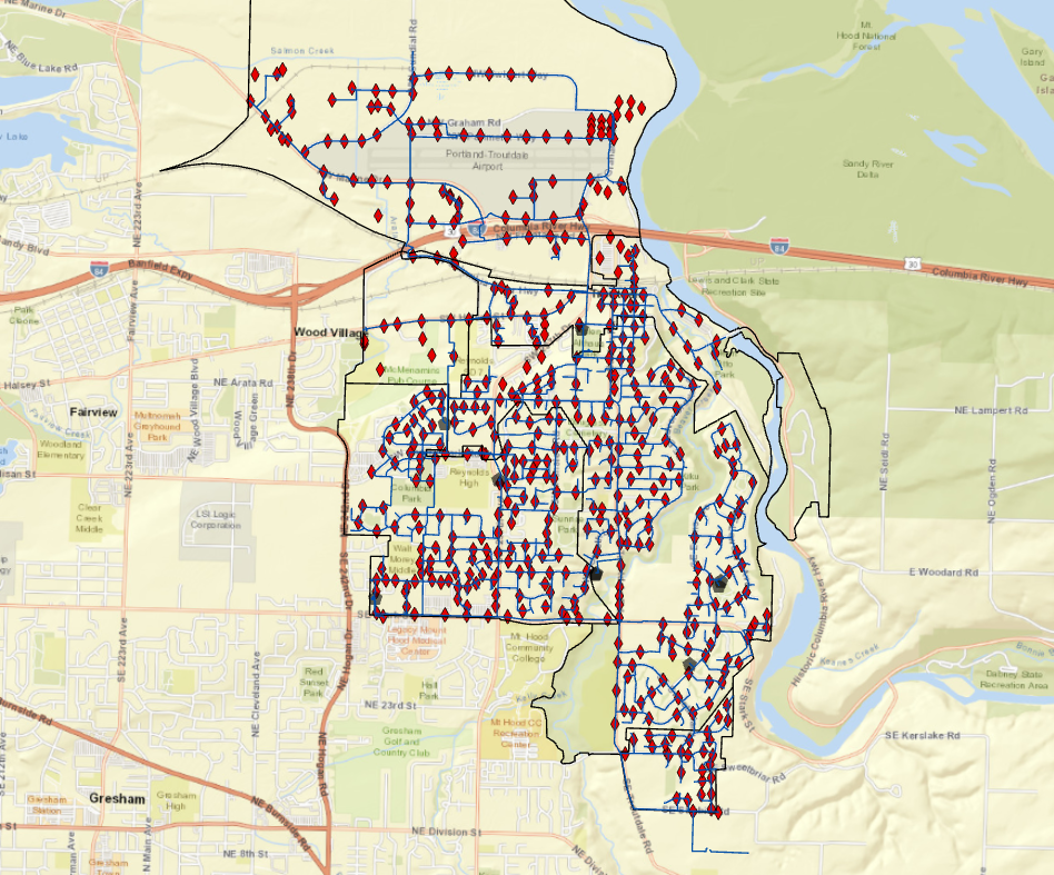
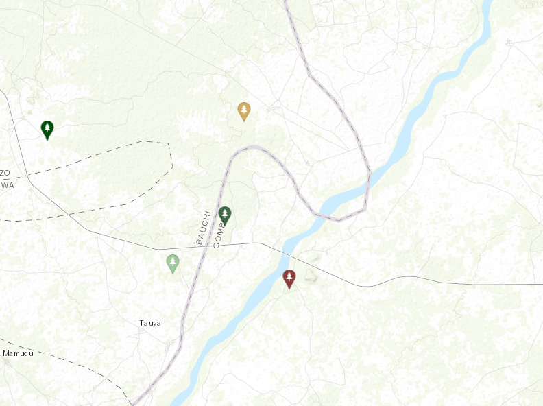
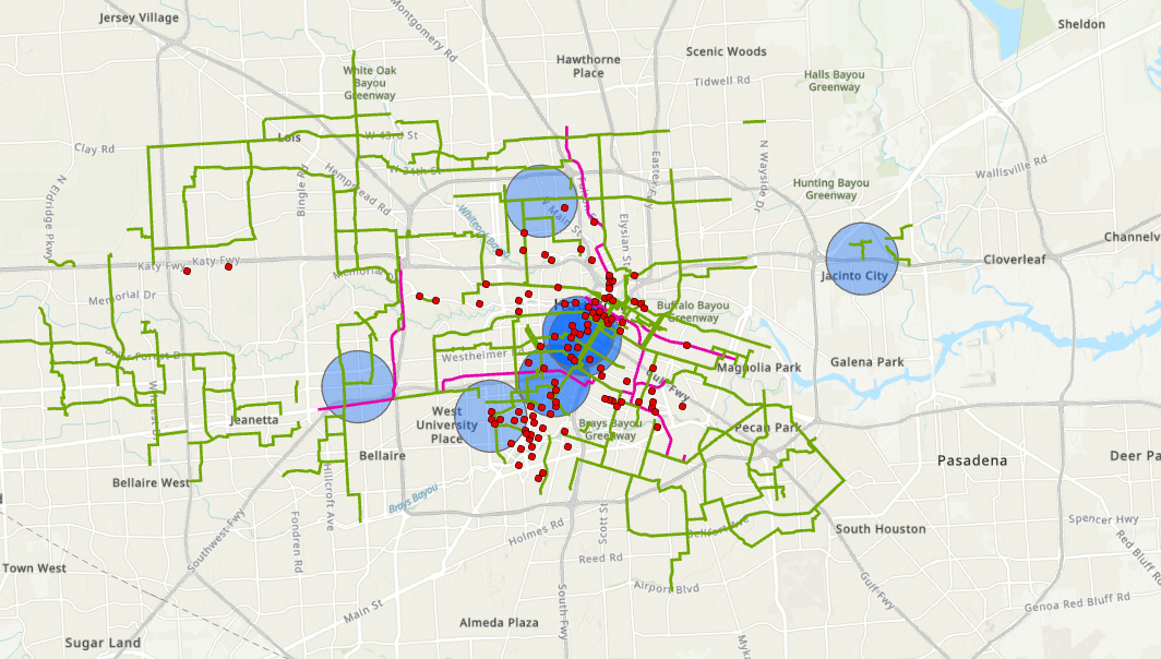
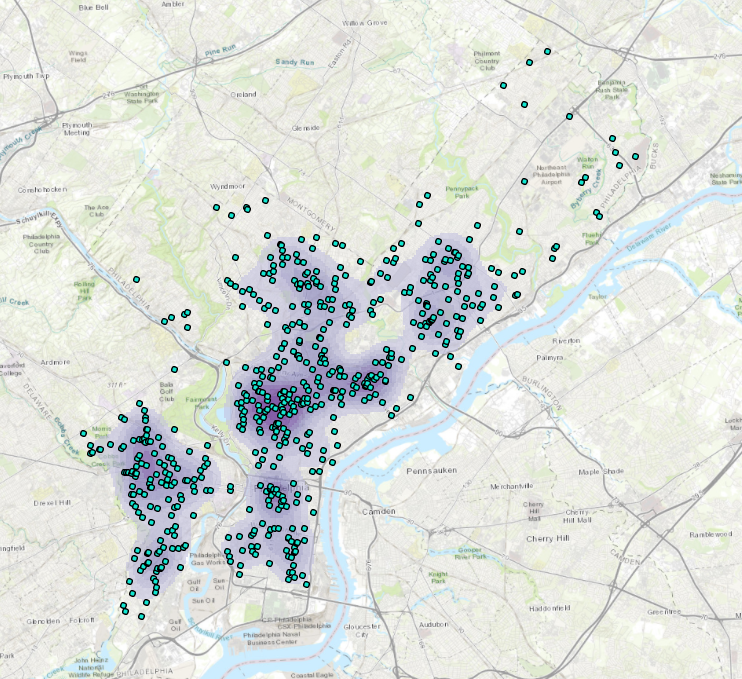
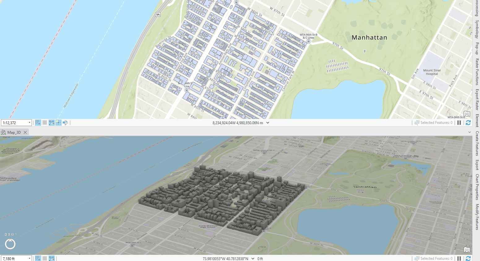
I have absolutely no idea why but when I save my map exports as PDFs it has the .pdf tab but it saves as a Chrome HTML?? When I open it it takes me to the PDF but why is it online? Here’s my map though (I should have probably made the map more zoomed in):

Weird PDF link: DelawareCountyMap

Screenshot of PDF:

 

 

 

Chapter 5

first step in tasks, I want to break down what I did. County is equal to South Sudan (only select South Sudan) and Year is >/= to 2011 (South Sudan data from 2011+). This task thing was very strange I’ve never used it before.

It was interesting learning tasks but I don’t think the text explained what this step was adding very well.

I prefer the model builder to the task route visually but the modelbuilder lacks the instructions given when using tasks so its a give and take. Here’s me running my model:

I haven’t started it just yet but I am scared to run Python code. I don’t want to run it I’d rather use the tasktool or modelbuilder >:(

When I tried to package my project I got a “conflict” saying that a geoprocessing item failed and it couldn’t package it. This was weird because I didn’t have any failed codes, but I fixed it by removing items with errors. I wasn’t feeling very extra so I skipped the “on your own” here where I check to see if this uploaded to my online account.

Chapter 6

Here is my created symbols for the trees:

It wouldn’t let me name the project “TreeInventory” for ArcOnline (it says the name is taken) so I added my name to the end “TreeInventoryFraire”.

My map for ArcOnlinne so far:

For the app thing, there is no app called “ArcGIS Collector” so I downloaded the first one that popped up called “ArcGIS Field Maps and it took  forever.

Well I downloaded it and then it said that I don’t have permission to use the app so I had to skip this part.

Attempt one at editing the new features attributes:

I got through his exercise but it was weird. I had to keep reopening my project because the program was losing its location and said it didn’t exist. I think this screwed with the portal linking to my online account because after refreshing and readding the layer it said that it couldn’t find it either. I think it might be because I had to give the online layer a different name since the map name was “already in use”.

Regardless, I now know multiple ways to edit maps from many devices!

Chapter 7

Starting off strong with more so actions like “join these two layers” instead of a step by step. Getting harder! Let me know I need to pay attention to what I’m doing more.

When I tried to save the locator it originally said that a parameter was missing. I think it was because I put “Houston_” and not “Houston_Locator”. File names are important (And annoying).

I don’t really understand what rematching did. I read the text and it’s still a little confusing. I have actually little to no idea what this did. Did it just match addresses that are the same but weren’t classified as the same?

My map after doing the merge, dissolve, and selected specific properties within the buffer:

When I opened the attribute table after the spatial join I only saw one row of data…I chose the wrong input for my spatial join! went back and fixed that annnndd it still looks the same D: Looking at the attributes of the buffer, it only shows one row of data as well.. I’m not really sure why this happened. My clipped layer and the following selection layer look fine in the attributes. Tried for a third time and it worked! I think I was selecting the wrong inputs, pay attention Logan.

Our pop-up menus look very different than the book.

My final map of this exercise with some selected prospective property locations, proposed/existing bike paths, and bike stations:

Chapter 8

My first map of robberies in January, how exciting:

I didn’t really consider the applications of GIS with crime. It obviously makes sense but it just adds another use of GIS for me.

Every time it says “run the tool” it reminds me of the artist group Run the Jewels 

negative points for bringing in the empirical rule and z-scores. Stats = no.

I hate this:

real vomit from all these cubes. It feels like the matrix:

I don’t want to work documenting crime spots, that’s for sure.

I did 8c and got the mods done. I just noticed that there is no topography for this scene. Not really a problem because I can work but odd:

Range and time on crime son (it’s playing in the picture so it looks a little empty right now):

Chapter 9

I started by extracting masks and mosaicing layers to make this property boundary:

Running the aspect tool and seeing the colors brings back trauma from remote sensing. I know these colors all correlate to the cardinal direction of the slope.

When adding the outline to the planting sites I made it purple instead of black because it was hard to see on the hillshade that was already greyscale and the slope added green/red. I promptly changed it back after adding the slope.

Here is my map with the property boundary, vineyard blocks, and planting sites. I also have on the 3pm hillshade shadow. There is limited area for planting on this property:

This modelbuilding reclassification probably won’t work. I don’t have a start and end column, only value and new.

My finished maps after raster calculator (which was being a little stinker). The dark red shows the most favorable planting sites within the black outline:

Chapter 10

My first map for 10a:

I didn’t have a symbol selection in my label ribbon. I had to right-click the layer and select labeling properties to get to the symbol tab it asked of me.

My created labeled map of Utah:

My finished layout of broadband speed/libraries in Utah County. (I have no idea why it made the pdf a html link? This has never happened to me before. I included a screenshot of the map because the link doesn’t even work.)

Layout1

 

Chapter 1
I didn’t expect the instructions to be so simple and linear. I figured it would ask me to do something instead of giving me step-by-step instructions down to the button to press.

My map after editing the public school symbology of the schools:

I funked around with the school walking areas and changed the color/added an outline. The outline helped me visualize where zones end but it does block up the map a bit with overlapping outlines. The color selection also feels inverted to human bias in color. The fact that the furthest walk is green is a bit confusing and should be considered if this map was ever used:

I added filters to the vision zero safety layer. These are going to minimize the amount of data points I see to only the selected expressions:

This next step required a little going astray from the book. It asked me to open the “clustering” tab but that doesn’t exist anymore, it has been renamed to “aggregation”. This is one of those reminders that things do update and change just a bit. But here’s my cute little clustered map of danger zones for pedestrians after it has been properly configured for fields:

Chapter 2

2.1

So far this work is super helpful for those who haven’t used ArcPRO before, but for those who have this feels like a drag. I understand starting from the bottom but some of this stuff is things I don’t even think about when I do them now.

I’m not sure if using the control key for selection is an Apple thing but I had to hold the shift button to select the 5 cities.

2.2

Opening the symbology tab was weird. I don’t often use the catalog tab as you have to manually open it to get to it. I can easily right-click the layer and select symbology. Just a reminder that there’s lots of ways to make something happen.

Here’s me messing around with distance measurements. The distance form Cape Town to Alexandria is 20,663.81 miles!

2.3

I’ve never made 3D images in Arc before, it looks so cool. Here’s my little linked map moment:

Chapter 3

I don’t like clicking the data tab to access the attribute table. I would rather right-click the layer to open it. The “new expression” button has also been changed to a “new clause” button instead. It’s weird though because it’s still labeled as expressions.

The export features have also changed. So I wasn’t allowed to save but not rename the output. So I just created it with the default name but renamed the layer. I’m not sure if it will show under this name in the file location but it worked.

I was really familiar with this exercise. I was reminded how finicky classes can be sometimes when you enter values. It makes me nervous.

Using the geoprocessing tools I found that the naming for double (double precision) didn’t exist anymore there was only double (64 bit). I had to do this step twice, because I wasn’t sure what went wrong but it came out right the second time. It was still a little wonky but it turned out with the same values.

Using the attribute table is a little extra mathy for me. I try to grasp what I’m doing but it’s difficult to understand sometimes.

Read the fine print, I couldn’t use the infographics tool until I was logged into ArcOnline. Weird but glad I caught it. Still couldn’t do the infographics. I used the correct login but it wouldn’t work and locked me out for 15 minutes… I got this far though! I had the map and percentage stats so this was the last step.

For the next exercise I was also having some troubles. When I imported the food deserts table layer, it was corrupted from the source. Google told me to repair the source but it said it was unavailable for the layer. After numerous location changes and removing and readding the file, it still didn’t work. Even opening it from the file to a new map it shows that it’s corrupted. So no stats here for me. I couldn’t do a spatial join either >:(

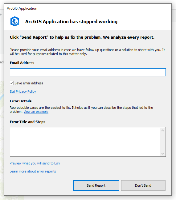
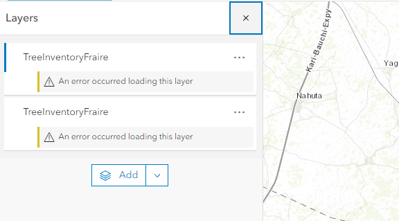
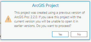
weird text I’ve never gotten  but got it saving the health data…I had to save it so I just updated it?

Chapter 4

my beautiful city water things map:

This city is safe, I repaired their waterlines:

My final map for chapter 4 after editing the water zones and highlighting it!:

Overall theses exercises taught me new things and reminded me how to do some older things. I only missed two steps due to being stuck but I wasn’t ever overly frustrated. Hopefully, this continues with our projects but we’ll see!

Chapter 4
Two ways to map density: by defined areas or by density surface.

defined areas: you can show and calculate density for the defined area. You can use a dot map.

density surface: created in GIS raster layers. Simple calculations are not as easy to read as weighted calculation in terms of rings. You can use graduated colors or contours to map density surfaces. Be aware of how many class you use, between 3-15 is the sweet spot, more or less gets confusing and loses data. Also note the colors you choose for the gradient and what appeals to the eye more (dark or light color gradient indicates high density).

Be cautious of how much info we need or don’t need, it’s a fine line between too much and too little info to not lose the obvious patterns in densities.
I remember calculating cell size conversions in remote sensing, it took such a long time. I think I left for lunch, used the restroom, got Rowley coffee and it still wasn’t done. I think I was converting points to tangible pixels with units but it’s crazy how much power and time it takes for these things sometimes.

This chapter was pretty short and covered a lot of things I knew how to do technically, but gave me more info on the use and reason behind these techniques. I liked comparing the dot and contour maps, I think it would be cool to do something with those in a project.

Chapter 5
to find out what’s inside, first build you area of study, and if its one or many.
I recall searching for feature attributes in remote sensing to narrow down a price range for potential house buyers. I also remember trying to import a boundary layer (shapefile) of Brazil and it kept not working. The datums were the same but it was not wanting to place itself properly. It took me 2-3 days to figure out how to do it.

Drawing areas/features: find whether features are in area or not. good for single area.
Selecting features in area: get a list of features in area, good for single area.
Overlaying areas/features: which features are in which areas and how many/how much in that area. good for multiple areas.

Most common summaries: count and frequency.
count: the total number of features inside the area, such as the number of businesses in a neighborhood.
frequency: the number of features with a given value, or within a range of values, inside the area, displayed as a table.

These slivers are very annoying. I remember making data points on a top layer that was slivered and when I flushed it out those data points were nulled because they didn’t fall in the area. I had to go back and move the points in just a hair to get them to be present.

The vector method provides a more precise measure of areal extent but requires more processing and postprocessing to remove slivers and to calculate the amount of each category in each area.

when choosing overlay to remove slivers: the raster method is more efficient because it automatically calculates the areal extent for you, but it can be less accurate, depending on the cell size you use. also prevents the problem of slivers. It is often faster because the computation that the GIS must do is simpler.
single area with one category: bar chart, or pie graph; multiple areas with one category: bar chart; multiple areas with multiple categories: histogram, cluster, or stacked bar chart, with few areas/categories you can use pie chart too

Chapter 6

I didn’t consider time or effort a cost in distance before this chapter.

Planar: calculating distance assuming the surface of the earth is flat

geodesic: taking into account the curvature of the earth when calculating distance

Inclusive bands: tells you the total number within bands as distance increases

distinct bands: lets you compare distance to other characteristics like how much someone 1000m away spends on groceries compared to 2000m.

I like the chapter setups where it introduces a concept, tells you its pros and cons, and also tells you how GIS does it as a function/what you need to do it, etc. Its helpful to have consistency. 

These few chapters have covered a lot of what was in our exercises for remote sensing. I had to do parcel selection within a given boundary to find homes for homebuyers that met their specifications.  I was reminded of this when it discussed selection within boundaries. I’m glad that a lot this is getting explained now. I would get pretty confused doing raster calculator calculations and not understanding what the numbers and symbols I entered meant. It is plugging in data into the calculator as a word problem too, the worst kind of math.

The spider diagram is cool, I like it. The graduated symbols map seems harder to read, the graduation of triangle size is hard to distinguish (for me)

The calculation of these distance seems like a really useful tool. I have worked with this concept a little bit but not to the extent that they went into in this chapter. I learned more about what Arc is doing behind the scenes in my random clicking and it makes things more comprehensive for me. I am more aware of why I’m doing something as opposed to just following directions to get it done.

 

Chapter 1

It’s kind of crazy how fast GIS is growing and how useful it is to know how to use it.

GIS analysis is a process for looking at geographic patterns in your data and at relationships between features.

I honestly struggle sometimes to come up with a research question when using GIS. It’s just such a large storage of data and the endless possibilities are daunting sometimes. It’s also really rewarding to look at your results at the end. Seeing your hard work mapped out and displaying data is super cool.

discrete: It is either there or it’s not, it can be pinpointed. continuous: Like rain/temperature they can be found/measured anywhere. areas enclosed by boundaries. summarized: represents counts or densities of individual features within a boundary (number of businesses in an area, total length of streams of watersheds)

When it started talking about summing certain data for an area I had setnull calculator flashbacks.  I’ve done vectors/rasters in Remote Sensing and I still don’t fully get it. Looking at the pictures it seems like vector is more cookie-cutter in its separation while raster looks gradual.  Figuring out how to overlay layers onto a pre-existing map with a coordinate system almost made me throw the computers last year. Brazil kept ending up in the middle of the ocean instead of overlaying on where it’s supposed to be.

Categories are groups of similar things.  can be represented using numeric codes or text. Ranks put features in order, from high to low. used when direct measures are difficult or if the quantity represents a combination of factors. Counts and amounts show you the total numbers. A count is the actual number of features on a map. An amount can be any measurable quantity associated with a feature.

Counts, amounts, and ratios are continuous values. Categories and ranks are not continuous values.

Chapter 2

This chapter so far reminds me a lot of the Importance of Maps course I took with Krygier. I think he said it’s not a class anymore? but it was based on a lot of map history and the bare structure/make-up of maps.

I also remember that assigning category values is annoying sometimes. The values just just from what you make them and the rules of how it works are really finicky (something for me to remember when doing this work).

why are all of these maps about crimes

At first, I didn’t think that 7 categories was a good max until it showed the map example with more than 7 and it felt very jumbled. This is something I will definitely keep in mind.

I didn’t have a ton of comments for this chapter, it felt very similar to what we learned in Maps so it was mostly a review. It talked about map projections and considerations when displaying maps. It went over the details of maps such as symbols, color, and width that can alter how a viewer perceives the map. I did mention above the few things I learned, but this chapter was also a lot more maps than Chapter 1. I do enjoy looking at them but it makes it harder to take notes sometimes.

Chapter 3

They mentioned the use of graduated colors or line width to show most to least values but this has always been a harder concept for me when making maps. I have a harder time differentiating symbols when they are just gradual transitions of themselves.

I think I have done ratios in ArcGIS and not realized. After reading this chapter I understand what I was doing a bit better now.

Counts and amounts show you the total numbers. Ratios show you the relationship between two quantities and are created by dividing one quantity by another, for each feature. Ranks put features in order, from high to low. Counts, amounts, and ratios are classes. Ranks are individual values.

Creating classes is also frustrating sometimes with Arc Pro. If data is unevenly distributed with gaps: natural breaks. If data is evenly disturbed and I want to emphasize the difference between values: SD or equal interval. If data is evenly distributed and you want to emphasize the relative difference of values: quantile.

I have never used a lot of these features in Arc. Some of them are really cool.

Hello, my name is Logan Fraire, I am a senior majoring in Zoology and Environmental Science with a Botany minor. I’m pretty involved with the ENVS Department, I am a member of the Student Board as well as the Student Department Manager on the Faculty Board. I really love nature and all the arts (books, fashion, applied, etc.). I’m super into plants and hope to work with them using remote sensing when I graduate 😀

Reading this chapter, it’s interesting to think that people wouldn’t be able to give a single example of GIS impacting their day-to-day lives. It just feels like such a prominent tool in my life that I wouldn’t be able to do a lot of things without it. I did agree that as an undergrad student, I knew what GIS was, but not a ton of how scientists use it for their research. (This text feels like they used big words on purpose to sound cool). When it talked about overlay and spatial analysis, it reminded me of Rowley telling us about how he had to manually overlay maps as an undergrad student. I often forget the times before tech and what that would have looked like so it’s always interesting to me to hear about these methods. I knew of ESRI but for some reason, I didn’t know it stood for Environmental Research Systems Inc. It’s also interesting to think of GIS as a new tool in Geography. It makes sense but to my knowledge, it is nearly fundamental for Geography and would be difficult to do without it. In the context of the chapter, I agree with Nancy Obermeyer’s view of GIS being as fundamental as a calculator. The chapter mentioned how GIS users don’t often question the result output from their technology and I related to this because I am also guilty of not questioning it. I just assume the system is right, like many other users. I agree that GIScience is foundational for GISystems, but it just goes well over my head to keep in mind sometimes. It’s interesting to question the relationship of GIScience/systems with humans. It makes me wonder what the evolving world of AI will do to GIS tech and our relationship with it. I knew about a lot of GIS applications, but not about G-commerce/business applications, very cool.

I looked into GIS applications and lizards. I found some cool work using GIS to model lizard habitat sites for research by Branch et al. Here’s a map of those habitat types:

I also found a cool study where they were trying to map the fundamental niche of a nocturnal gecko species using internal, environmental, and climatic data gathered in their work. They used GIS tech to run many models to understand where these geckos might be active in Australia based on multiple factors. Here’s an example of some of those models:

caption: Fig 4: Results of continent-wide 0.05°-resolution biophysical simulations for the physiology of EA6 male Heteronotia binoei for (a) degree-days for egg development, (b) potential activity time, (c) maintenance metabolic costs, (d) food requirements per hour of activity, (e) water loss, and (f) discretionary water. All maps are of annual summations. The dotted line represents the known southern distributional limit of H. binoei”

Branch, L. C., Hokit, D. G., Stith, B. M., Bowen, B. W., & Clark, A. M. (1999). Effects of landscape dynamics on endemic scrub lizards: an assessment with molecular genetics and GIS modeling. Florida Game and Fresh Water Fish Commission.

Kearney, M., & Porter, W. P. (2004). Mapping the fundamental niche: physiology, climate, and the distribution of a nocturnal lizard. Ecology, 85(11), 3119-3131.