Author: jrdemaggio

Zip Code: This data set contains all of the zip codes inside of Delaware County.  In 2003, Delaware County zip codes were carefully evaluated and cleaned-up based on cross-referencing between the Census Bureau’s zip code file from the 2000 census, the United States Postal Service website, and tax mailing addresses from the treasurer’s office. The zip code layer was then created in 2005 by dissolving all Delaware County parcels by their property addresses.

Recorded Document: This data set has specific points representing recorded documents in the Delaware County Recorder’s Plat Books, Cabinet/Slides, and Instruments Records which are not represented by active subdivision plats. They are documents such as; vacations, subdivisions, centerline surveys, surveys, annexations, and miscellaneous documents within Delaware County, Ohio.

School Districts: This data set consists of all School Districts within Delaware County, Ohio. The data was originally created via the Delaware County Auditor’s parcel records of the school districts. This dataset is updated on an as-needed basis and is published monthly.

Map Sheet: This dataset consists of all Delaware County, Ohio map sheets.

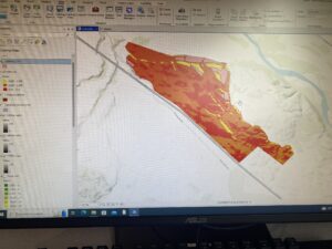
Farm Lot:  This data set consists of all the farm lots in both the US Military and the Virginia Military Survey Districts of Delaware County. The dataset is maintained on an as-needed basis where new surveys have been recorded.

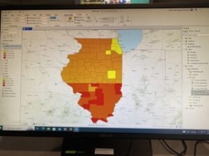
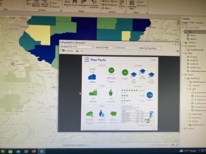
Township: This data set consists of 19 different townships that make up Delaware County, Ohio. This dataset is updated on an as-needed basis and is published monthly.

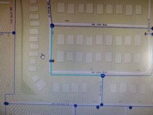
Street Centerline: The State of Ohio Location Based Response System (LBRS) Street_Centerlines depict the center of pavement of public and private roads within Delaware County. It is intended to support appraisal mapping, 911 emergency response, accident reporting, geocoding, disaster management, and roadway inventory that conforms to Ohio Department of Transportation Roadway Inventory Standards.

Annexation: This data set contains Delaware County’s annexations and conforming boundaries from 1853 to the present. This dataset is updated on an as-needed basis once an annexation has been recorded with the Delaware County Recorders office. It is published monthly.

Condo: This data set consists of all condominium polygons within Delaware County, Ohio that have been recorded with the Delaware County Recorders Office.

Subdivision: This data set consists of all subdivisions and condos recorded in the Delaware County Recorder’s office. This dataset is updated on a daily basis and is published monthly.This data set consists of all subdivisions and condos recorded in the Delaware County Recorder’s office.

Survey: Survey points is a shape file of a point coverage that represents surveys of land within Delaware County, Ohio. These surveys are found in documents in the Recorder’s office and the Map Department.

Dedicated ROW: This data set consists of all lines that are designated Right-of-Way within Delaware County, Ohio. This dataset is updated on a daily basis and is published monthly.

Tax District: This data set consists of all tax districts within Delaware County, Ohio. The data is defined by the Delaware County Auditor’s Real Estate Office. Data is dissolved on the Tax District code.

GPS: This dataset identifies all GPS monuments that were established in 1991 and 1997. This dataset updated on an as-needed basis, and is published monthly.

Original Township: This dataset consists of the original boundaries of the townships in Delaware County, Ohio before tax district changes affected their shapes.

Hydrology: This dataset consists of all major waterways within Delaware County, Ohio. This data was enhanced in 2018 with LIDAR based data. This dataset is updated on an as-needed basis and is published monthly.

Precinct: This dataset consists of Voting Precincts, and is maintained by the Delaware County Auditor’s GIS Office under the direction of the Delaware County Board of Elections.

Parcel: This dataset consists of polygons that represent all cadastral parcel lines. Information or attributes regarding individual parcel records is maintained in the Auditor’s CAMA (Computer Aided Mass Appraisal) system.

PLSS: This data set consists of all the Public Land Survey System (PLSS) polygons in both the US Military and the Virginia Military Survey Districts of Delaware County. This data set was created to facilitate in identifying all of the PLSS and their boundaries in both US Military and Virginia Military Survey Districts of Delaware County.

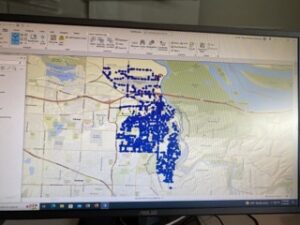
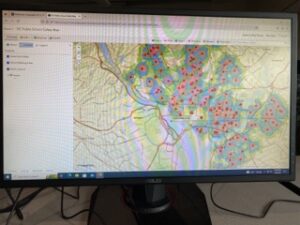
Address Point: The Address_Points data set is a spatially accurate representation of all certified addresses within Delaware County Ohio. The Address_Points layer is intended to support appraisal mapping, 911 Emergency Response, accident reporting, geocoding, and disaster management.

 

Chapter 6: Chapter six focused on collaborative mapping as well as putting in data by hand through ArcGIS’s app, which I thought was fun to explore. For me, chapter six was pretty laid. back.

Chapter 7: Chapter 7 was focusing on Houston, TX, and its roads and bike paths throughout the city where we learned how to rematch/correct different addresses as well as use buffers, There weren’t any bugs for me in this chapter either so it was easy to explore different ways to do what the book was teaching us.

 

. 

 

Chapter 8: Chapter eight had a lot of bugs for me which was frustrating, however, it still was a very insightful chapter. It was interesting when I learned how to separate the robbery points by time, similar to when we looked at the health of Illinois over several years. Using kernel density to find relations between the area and its crime rates was also interesting.

Chapter 9: This chapter gave me some trouble in the beginning, but I found out it wasn’t the files it was just user error, and then was able to move past and explore, overall this chapter was very fun in my opinion.

 

 

 

 

 

 

Chapter 10: Chapter ten was fine until exercise 10c where we had to format the two different maps onto a layout and publish it. I didn’t have many problems other than the distance markers, I tried several timesto configure them the way the book wanted and it never came out right, so I moved past that part and published the maps anyways.

Chapter 1-

Chapter one was basically going over the basics of GIS. We went over basic map symbology and how to change and manipulate a features symbology to better fit the needs of our map. Chapter one, unlike the other chapters, had us work with ArcGIS online rather than ArcGIS Pro. I assume it’s to help us get familiar with basic functions and features that we end up using in the proceeding chapters. Some key terms that were covered we vectors, rasters, and attributes.

Chapter 2-

Chapter 2 went more in-depth into topics and terms that we’ve gone over in previous readings. Some of the main objectives we had were to go over more of the basics such as importing map documents, examining and exploring the contextual ribbon, and selecting features. That was primarily in 2a, however, in 2b we started to label features, and base-maps, as well as package and share the maps. Chapter 2c was especially new as it involved creating a 3D scene for the first time and getting familiar with its functions. I thought this chapter was especially fun because it was my first time working with ArcGIS Pro. I, unfortunately, forgot to take pictures of the work.

Chapter 3-

Chapter 3 was one of the more challenging chapters for me in terms of bugs and information that I needed not being included, so I had to skip a step or 2 during the exercises. 3a went into topics like adding additional data to a map, and selecting features by certain attributes. 3b was very intensive on using data tables, as well as using the swipe function. Using the swipe function with separate layers was probably one of the most vital skills I learned during this chapter. Instead of turning off and on different layers of the same area over a period of time I was able to use the swipe function and was able to see a more distinct difference between the different counties that we were analyzing in Illinois. It was easier to see the change and progress over time,

Chapter 4-

Chapter 4 was equally challenging because of technical bugs and whatnot. Chapter 4 was the smallest scale map we had worked with so far, making all of the exercises more precise. This chapter dealt more with specific positions and using x,y coordinates and attribute domains. Towards the end of the chapter in 4c was where I had the hardest time, but it was the most growth I had experienced throughout chapter 4; using and editing different polygons on maps was the most frustrating this I have done so far, but I did eventually get it down. There were also other steps we had previously done that were implemented into this chapter such as linear features that gave us a function we’ve already learned, but used it within a different context, which I thought was useful.

Chapter 5-

Chapter 5 was very beneficial and unlike chapters three and four, didn’t have any complications. We were given one map layer of conflict within Africa, and throughout the chapter learned to make one base-map layer into several different layers and isolating them into individual countries within Africa. The book had us go through definition queries that allowed us to isolate the layer into one area and one specific conflict, such as riots/protests or violence against civilians. There was also another emphasis on the symbology of a layer, more specifically on graduated symbols to show different concentrations of a specific feature. Towards the end of the chapter we had begun to create new layer files by using Python to script them, which honestly was difficult at first but I can see it becoming a very useful skill later on.

Chapter 5

Chapter five teaches about “finding what’s inside” and how it lets you see whether an activity occurs inside an area or summarized information. When paired with multiple areas, you can compare them to see patterns and information that you weren’t able to see beforehand. The main focus of this chapter was discussing boundaries that can isolate locations or information to create summary data. You can do this with a single area, which allows you to summarize information and monitor the area. You can also set boundaries on several areas that you would then treat as one. An example Mitchell uses for setting a boundary around multiple locations is if you want to find out the number of businesses within a group of zip codes. It’s important to know that you’ll want to be able to identify each area uniquely, or else you or your audience wouldn’t be able to understand the information presented. You can do this by using names or even numbers to set one area apart from another. Mitchell then talks about using counts, lists, and summaries within a boundary to gather all of the features that you’re looking for within a boundary. Another important factor in mapping with boundaries is whether you decide to include only features that are completely inside your boundary, or if you want to include features outside as well. It’s effective if you choose the latter to use different colors to distinguish the features inside from the ones outside. There are also many methods to go about mapping what’s inside; drawing areas and features is good for finding out whether features are inside or outside an area, selecting the features inside the area is good for getting a list or summary of features inside an area, overlaying areas and features is good for summarizing how many or how much by area. As with the rest of this book, this chapter provides a list of ways to map and present the information you’re studying.

Chapter 6

Chapter 6 talks about finding what’s nearby and how it lets you see what’s within a set distance or travel range of a feature, allowing you to monitor events inside an area. First, Mitchell talks about determining the style of analysis, which mainly includes travel cost and distance, but also talks about planes and whether what you’re analyzing requires taking the planet’s curvature into account. Travel range specifically is measured using distance, time, or cost: finding the traveling range of a feature can help define the area served by a facility and can help delineate areas that are suitable for, or capable of supporting, a specific use. When talking further about cost, Mitchell states that time is one of the most common costs, along with money or effort expended, in which all of these costs describe the term “travel costs”. He then talks more about calculating distance in two different ways, either assuming that the Earth is flat, or if you’re taking into account the curvature of the Earth, which are respectively known as the planar and geodesic methods. The planar method is more efficient when your area of interest is smaller, such as a city, county, or even a state. The geodesic method is more efficient when your area of interest is a large region, continent, or even the entire Earth.  The chapter then goes back to boundaries and talks about inclusive rings, which are useful for finding out how the total amount increases as the distance increases when specifying more than one area. You can also use district bands, which are useful if you want to compare distance to other characteristics in your map. From here we move on to tree different ways to find what’s nearby, straight line distance, distance/cost over a network, and cost over a surface, which all have their own intended purposes.

Chapter 7

The final chapter for Mitchell’s book talks about map changing. Map changing is when you map in GIS where things move, or the changing conditions in a place over time. Knowing what’s changed in an area, or multiple areas, is useful when understanding how things behave over time, anticipate future conditions, or evaluate the results of an action or policy. A common example of map changing is mapping the paths of hurricanes to see whether the patterns change from month to month. By mapping conditions before and after an event, you can see the impact of it, and just like in the first chapter, this helps you determine where you need to take action. I feel that defining the analysis for this kind of mapping is crucial (just like when defining analysis in other chapters) because you can either go about it by showing the location and condition of features at each date, or you can calculate and map the difference in a value for each feature between two or more dates. You can see geographic changes in location or in character or even magnitude, and choosing one or the other can alter the appearance of your map, therefore it’s important define your analysis. When mapping change by location you can see how a certain feature behaves, which can help you predict where they’ll move, and mapping change in character or magnitude shows you how conditions in a given place have changed. From here the chapter moves onto focusing on measuring by time, where it gives you a list of  ways you can measure time: by a trend (change between two or more dates/times), by “before and after” (analyzing conditions preceding and following an event), and a cycle (a change over a recurring time period, such as a day, month, or year). The chapter then talks about knowing what information you need in order to map change effectively. To me this might be the most difficult thing to learn when we start using ArcGIS more, but I’m excited to see what patterns I can create and form with map making.

 

Chapter 1

In this first chapter, Mitchell introduces GIS analysis as a whole, explaining the process one needs to follow to use GIS programs like ArcGIS efficiently and the best way to present your data. You need to know what question you’re asking, what information is required to answer your question, understand the data you have as well as choose a method to map your data that represents your findings the clearest. Your results can either be mapped as discrete or mapped as continuous, or even mapped as a summary of areas. However, while all three approaches are using the same data, the end results of both methods will be different, making it important for you to choose the method that will convey what you’re presenting the clearest. Mitchell also walks us through the differences between vector models and raster models, saying that with vector models, “each feature is a row in a table, and feature shapes are defined by x,y locations in space”, and those areas are defined by borders and are represented by closed polygons. From there he explained that with the raster model, locations aren’t defined by specific coordinates but rather with matrices of cells in continuous space and that the sizes of the cells can be altered to fit the data that you have, which he goes further in-depth later on. From there he lists different types of attribute values such as categories, ranks, counts, amounts, and ratios. Categories are groups of similar things, ranks put features in order from high to low, counts and amounts show total numbers, and ratios show the relationship between two quantities. This was a lot of information to try to retain, especially for this being my first time diving deep into GIS analysis, but in the following chapters, each definition and feature are further explained, aiding me in my understanding of it all.

Chapter 2

Chapter 2 talked about mapping where certain things are, such as crimes, businesses, employees, etc. When asked the question of “why” it seems obvious for the reason to look at a map is to see where a certain feature is. While that still remains true, mapping where things are helps make patterns noticeable and from there you can decide where you need to take action. An example of this in the textbook is when you map where certain crimes (burglaries, theft, auto theft, assault) occur in a specific area. From there you can see where they all have occurred, and see patterns in where there are more crimes in one area in another, as well as where certain crimes are more likely to occur. This is made possible by starting with a basic map with all of the same symbols, from which you can move to divide the feature into different categories, making your data points more specific by either using different symbols or different colors. Mitchell then dives into how you use your map and states that it is paramount when creating a map, to make sure that the map is appropriate for the audience you’re addressing as well as the issue that you are addressing. If your audience isn’t familiar with the area you’re representing, it’s good to add reference locations such as major roads, lakes, or administrative boundaries to provide more context to your map. Not only are reference locations important, but so is the amount of categories you decide to use. If you use too many categories the patterns in the map can become too complex to see, however, if you include too few categories, essential information can be lost. The same thing goes for symbols, it is easier for people to discern between different colors than different symbols if there are enough points of data that are clustered together. The end goal for your map is to convey the patterns and information you desire in the clearest and most efficient way possible. 

Chapter 3

This chapter focused primarily on quantitative data and was by far the most when it comes to information overload for me. Early in this Mitchell states that mapping the most and the least allows you to compare places based on quantities, which can help bring out patterns and a better understanding of the relationships found in your data. From this basic understanding, the next step is to understand the three features and what they each entail, where discrete features are individual locations, linear features, or areas, continuous phenomena as defined areas, and data summarized by shaded areas. The theme of the audience is revisited in this chapter and the discussion of how the appearances of maps differ between the exploration and the presenting of the data you study. If you are simply exploring your data, then your map should be more detailed as well as mapped in various different ways. If you are presenting the map and data, your map should obviously be more specific with the relationship you’re attempting to prove to your audience. From there the chapter dives back into the different attribute values, where I learned more about the use of ratios. Ratios in this chapter were very important when it came to displaying the highest and lowest values of data, and especially important when it comes to shaded areas on a map. Ratios help generate the differences between large and small areas. This can be especially useful when it comes to finding proportions and densities, which are talked about in chapter four. Counts, amounts, and ratios are usually grouped into classes because each feature in your map can have different values, especially when the range of values you have are larger. When creating classes it’s important to know where each feature will lie in your classes, because if you change the classes of your map, the map can look very different from the one before. We then go into the different kinds of class breaks. Natural breaks are where classes are based on natural groupings of data values, quantile is where each class contains the same amount of features, an equal interval is where the difference between the high and low values is the same for every class, and standard deviation is where features are placed in classes based on how much their values vary from the mean. They all operate differently, meaning that they all have their advantages and disadvantages which can make it difficult to decide which class type will be most effective in appropriately displaying your data.

Chapter 4

Chapter four is completely on map density, which in the beginning states what it is and what it does: mapping density can show the highest concentration of a feature you’re examining, it can be more efficient than just mapping locations, and it’s good for census tracts and counties. However, there is a difference between the two methods of mapping density, by defined area and by density surface. When you go by a defined area, you can use a dot map or calculate a density value for each area, which allows you to see density graphically. When calculating the density value of each area, “you divide the total number of features, or total value of the features, by the area of the polygon” and from there each area is then shaded based on its density value. When mapping density value it’s best to use different shades of a color, typically the lightest shade indicating the lowest density and the darkest shade representing the highest density value. When mapping by density surface it is usually created in the GIS as a raster layer, which we learned in chapter one as matrices of cells in continuous space. The benefit of mapping by density surface is that it provides the most detailed information in comparison to mapping by defined area, however, requires more effort to do. It was nice that there were tables included in this chapter that stated when to use one or the other; you should map density by area if you have data already summarized by area, or lines/points that you can summarize, and you should map density by surface if you have individual locations, sample points, or lines. I feel that most of the time when mapping density it would make more sense to map the densities by shaded areas rather than graphing dots because, for me personally, it’s easier to distinguish the difference between color shades as opposed to clusters of dots, because the clusters can then further skew the true value of density being portrayed on your map. Cell size and search radius also play roles in how your map and presented patterns appear. If your cell sizes are smaller, you’ll have a smoother display, and if your cell size is larger you’ll get a coarser image. The typical range of cell sizes to use is between 10 and 100 cells per density unit. With a search radius, the larger the search radius, the more generalized the patterns in the density surface will be, while a smaller search radius shows more local variation, but you have to be careful because if your search radius is small enough, most cells will have very low-density values, creating, “broader patterns in the data may not show up.” In all of this reading, I have learned that many factors in GIS mapping are a range or a scale, and it’s up to you to find the right proportions that will bring the most fruition to your map.

Hi Krygier! You already know who I am from last semester, but my name is Jacob DeMaggio and I am a freshman here from Saint Louis, Missouri. I am an Environmental Science majorr (possibly a double major in Zoology) and additionally a Spanish minor.

When reading Schuurman ch. 1 I thought it was very insightful how at the beginning of the chapter the author addresses the matter that GIS has multiple identities based on who the user is and what questions they’re asking. To me, it not only showed how GIS can have multiple different “identities” but also how there is no exact way to pinpoint a definition of GIS that everyone will agree upon.  Additionally, I found it interesting when there was a brief discussion on what spatial analysis is and how it differs from mapping and GIS, how it extracts more data and information than can be gleaned by map data. I specifically find this interesting because I would always think that spatial analysis would be the same as mapping data. I also find it interesting that there were multiple different people, from multiple different areas (the U.S., Canada, and the UK) and how many people believed that the development of GIS was inevitable. It started to make me think about how our world today would be different if we didn’t have GIS, and it made me realize how much we use it on a daily basis in our cars every day, and for us to not have had that would have made everyone’s lives so much worse, which showed me how grateful I am to be in a time where GIS does exist. On page 7 the author quotes someone that uses an analogy of GIS and a calculator and helped make more sense of GIS. The analogy was that both are fairly straightforward and clear-cut as to what they do, but you have to understand all of their functions and intricacies of them before being able to effectively use them. It also has been shown throughout the reading that it is evident that there is a difference between the quantitative implications of GIS as well as the cartographic implications of GIS and also the relationship between the two of them.

When looking for GIS applications, I looked at the application for members of the LGBTQ community, and it discussed how with GIS we are able to make relationships between sexuality, place, and space. It goes deeper into how “queer space transgresses the normative and challenges (hetero)sexualized space”. Another GIS application I looked at was for crime-related GIS applications and I found that you can us GIS to create a map that can identify where the crimes are occurring and clarify what crimes are or are not related based on your research, which in turn can allow investigators to target their efforts and line officers to patrol and respond to locations while being more fully aware.

Sources:

https://community.esri.com/t5/conservation-gis/why-should-gis-matter-to-queer-people/ba-p/1011618

https://www.esri.com/content/dam/esrisites/sitecore-archive/Files/Pdfs/library/brochures/pdfs/crime-analysis.pdf