Month: February 2023

1)GIS has 5 parts: hardware, software, data, procedures, and people. It manages, captures, and stores data. Spatial data is information that represents real world data. Attribute data is information about spatial data.

Base maps are provided by arcGIS online. it increases the accessibility of GIS and map making/spatial analysis.

Web maps allow information to be retally available to many people at once. On a similar note the open data movement provides the public with accurate data.

Point, line, and polygon data is called vector data.

Things that are similar can be grouped into layers on a map.

Raster is recorded or measured data for any location on the surface to form a digital surface.

2)simple technical elements of GIS: map, analysis, insert, and view.

context planes allow you to modify the map

Shows how to connect folders to maps

3)created multiple layers to compare the differences.

Talks about data relations

Changing attributes

4)using and creating geodatabase

learned how to limit geodatabase highlighting information I think is relevant

Create lines and polygons

5)played with commands, reminds me of coding in high school

Use tasks

Enjoyed the more technical side of gis

 

 

 

 

 

 

Once I worked past all the bugs I enjoyed getting to use the software and I found that there were somethings I could figure out without the book just by poking around. I enjoyed the work i could do with the data tables and reminds me of the coding class I took in high school. I wasn’t able to get the 3d model to work but I was able to work through most of the other stuff. I will take more screen shots in the next chapters I was quite focused on getting the work done.

Zip Code: Contains all zip codes in Delaware County. Created in 2005 by dissolving all parcels in the county by property address with tax exempt parcels and dedicated roads with no zip codes being manually populated. Published monthly.

Recorded Document: Contains points that represent recorded documents in the Delaware County Recorder’s Plat Books, Cabinet, Slides and Instrument Records not represented by subdivision plats that are active. Documents such as vacations, subdivisions, centerline surveys, surveys, annexations and miscellaneous documents. Updated on a weekly basis and published monthly.

School District: Contains all school districts within the county. Created via the Delaware County Auditor’s parcel records of the districts. Updated on an as-needed basis and published monthly.

Map Sheet: Contains all of the map sheets of Delaware County. A map sheet is a single map or chart in a map series, such as a USGS 7.5-minute topographic map, or printed map.

Farm Lot: Consists of all the farm lots in both US Military and the Virginia Military Survey Districts of Delaware County. Data is maintained on an as-needed basis where new surveys are recorded.

Township: Consists of 19 different townships that make up Delaware County. Dataset is updated on an as-needed basis and published monthly.

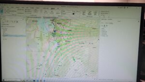
Street Centerline: Contains a spatially accurate topologically correct representation of the road system in Delaware County. Depicts center of pavement with public and private roads with address range data developed from data collected by field observation of existing address locations and manual addition from building permit information. Supports appraisal mapping, 911 emergency response, accident reporting, geocoding, disaster management and roadway inventory given to ODOT Roadway Inventory Standards. Updated on a daily basis for all fields but 3D, and published monthly. 

Annexation: Contains Delaware County annexations and conforming boundaries from 1853 to present day. Updated on an as-needed basis and published monthly.

Condo: Consists of all condominiums within Delaware County.

Subdivision: Consists of all subdivisions (which there’s a lot of) within Delaware County. Updated on a daily basis and published monthly.

Survey: Shapefile of land surveys in Delaware County using point coverage. Old surveys have been scanned from the map department and added in. All surveys after May 2004 were and are being scanned by the map department. Updated on a daily basis and published monthly.

Dedicated ROW: Consists of all lines that are designated Right of Way within Delaware County. Updated on an as-needed basis and published monthly.

Tax District: Consists of all tax districts in Delaware County and defined by the Delaware County Auditor’s Real Estate Office and dissolved on the Tax District code. Updated on an as-needed basis and published monthly.

GPS: Consists of all GPS monuments established between 1991 and 1997. Updated on an as-needed basis and published monthly.

Original Township: Similar to the township layer, but only using the original townships from Delaware County. Updated on an as-needed basis and published monthly.

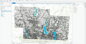
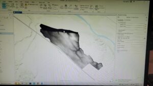
Hydrology: Contains all major waterways in Delaware County, enhanced by LIDAR data in 2018. Updated on an as-needed basis and published monthly.

Precinct: Consists of all voting precincts in Delaware County. Maintained by the Delaware County Auditor’s GIS Office with the direction of Delaware County Board of Elections. Updated on an as needed basis and is published as needed by the Delaware County Board of Elections. 

Parcel: Consists of polygons that represent parcel lines of Delaware County, maintained by the Delaware County Auditor’s GIS Office. Represented by recorded documents in the Delaware County Recorder’s Office. Maintained on a daily basis and published monthly.

PLSS: Consists of all Public Land Survey System polygons in both the US Military and Virginia Military Survey Districts of Delaware County. Maintained on an as-needed basis where new surveys have been recorded, updated on an as-needed basis and published monthly. 

Address Point: State of Ohio Location Based Response System Address Points dataset is spatially accurate representation of all addresses in Delaware County. Maintained by Delaware County Auditor’s GIS Office. Intended to support appraisal mapping, 911 emergency response, accident reporting, geocoding and disaster management. Updated on a daily basis and published monthly. 

Building Outline: Consists of building outlines for all structures in Delaware County. Created in 2008 from Orthophotos. Updated on an as-needed basis and is published monthly.

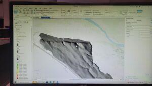
Delaware County Contours: Consists of two-foot contours to show topographical and elevational changes in Delaware County.

 

Chapter 6:

6A. Set up a domain, set up a feature class fields, symbolize features, publish features

– tree inventory shared file in “TreeInventory3” :/

6B. create a map, set up additional data display options, share a map & 6C. start ArcGIS collector, collect a tree location and enter the data, view the map in arcGIS pro.

-finished the map on my phone onto chapter 7 🙂

Chapter 7:

7A. Join a table, symbolize using graduated colors

7B. Create an address locator, Geo code addresses, Rematch Addresses & 7C. Create buffers, Merge and dissolve features, Clip Features, Select by attribute and location, Create a spatial join

Chapter 8:

8A. Select by attribute, Create a kernel density

The data did not transfer properly so for steps 10-15 the steps had to be modified so that the layer could be created and the kernel density could be created.

8B. Run the Optimized Hot Spot Analysis Tool, Create a space-time cube, Visualize a space-time cube, Run the Emerging Hot spot analysis tool.

8C. Switch to a local view, change 3D visualization styling & 8D. enable time, animate using the Time slider, Animate using the range slider

Chapter 9:

9A. convert a line feature to a polygon feature, clip rester layers, merge rasters

9B. Derive an aspect surface, derive a slope surface, Derive a hill shade surface, Visually compare analysis outputs,

• nothing is completely in shadow right now.
• 4 planting sites have mostly low slope topology
• one planting site has some land facing either south, southwest, or southeast.
• none of the planting sites are in shade at this time
• yes we can identify planting sites that would have enough sunlight in the afternoon and would be best

9C. reclassify criteria rasters, combine criteria rasters.

• Greenfield fine sandy loam soil from 9-15% slopes, xerorthents and loamy soil, and rincon clay loam soil with 15-30% slopes
• some potential sites have been planted

Chapter 10:

10A. create a definition query, fine tune the symbology, apply symbol layer drawing

• There are 3 areas of fixed wireless technology

10B. label features using the Maplex label engine

10C. add a layout to the project, insert map frames, insert a legend element, insert a scale bar, insert a north arrow, insert dynamic text, a title and rectangles

10D. export a layout to a PDF file, save a layout file, package and share a project template.

I finished!!

• Zip code: This dataset contains all zipcodes within Delaware County, Ohio. These zip codes were carefully evaluated in 2003 and cleaned up based on the Census Bureau’s zip code file from the 2000 census. 
• Recorded Documents: This dataset contains points that represent recorded documents in the Delaware County Recorder’s Plat Books, Cabinet/Slides, and Instrument Records. 
• Farm Lot: This dataset contains all the farm lots in the US Military and the Virginia Military Survey Districts of Delaware. 
• Township: This dataset contains 19 different townships that make up Delaware County.
• Street Centerline: This dataset contains the data on the center of pavement of public and private roads within Delaware County. It intends to support appraisal mapping, 911 emergency response, accident reporting, geocoding, etc.
• Annexation: This dataset contains Delaware County annexations and conforming boundaries from 1853 to the present. 
• Condo: This dataset contains all condominium polygons within Delaware County, OH. 
• Subdivision: This dataset contains all subdivisions and condos recorded in the Delaware County Recorder’s Office.  
• Survey: Survey points is a shapefile of a point coverage that represents surveys of land within Delaware County.
• Dedicated ROW: This dataset contains all lines that are designated Right-of-Way within Delaware County, OH. This data is line data that is created through the daily updates of Delaware County’s Parcel Data. 
• Tax District: This dataset contains all the tax districts within Delaware County, OH. 
• GPS: This dataset identifies all GPS monuments that were established in 1991 and 1997. It is updated based on need and published monthly. 
• Original Township: This dataset contains the original boundaries of all the townships in Delaware County, OH. 
• Hydrology: This dataset contains all the major waterways within Delaware County, OH. 
• Parcel: This dataset consists of all Parcels within Delaware County, OH. 
• PLSS: This dataset contains polygons depicting the boundaries of the two public land survey districts within Delaware County, OH. 
• MSAG: This dataset contains the boundaries of the 28 different political jurisdictions, such as townships, cities, and villages that make up Delaware, OH.
• Municipality: This dataset contains all municipal boundaries in Delaware County, OH.
• Address Point: This data is maintained by the Delaware County Auditor’s GIS Office. This dataset represents all certified addresses in Delaware County. OH. 
• Building Outline: This dataset contains building outlines for all the structures in Delaware County, OH. It was last updated in 2018. 

• Zip Code – This data set contains all zip codes within Delaware County, Ohio…This layer was also used to populate the zip_right and zip_left attributes for Delaware County’s road centerline.
• Recorded Document – This dataset consists of points that represent recorded documents in the Delaware County Recorder’s Plat Books, Cabinet/Slides and Instrument Records which are not represented by subdivision plats that are active. They are documents such as; vacations, subdivisions, centerline surveys, surveys, annexations, and miscellaneous documents within Delaware County, Ohio.
• School District – This data set consists of all school districts within Delaware County, Ohio.
• Map Sheet – This dataset consists of all map sheets within Delaware County, Ohio.
• Farm Lot – This dataset consists of all the farmlots in both the US Military and the Virginia Military Survey Districts of Delaware County.
• Township – This data set was created to facilitate identifying the geographic boundaries of each township within Delaware County, Ohio.
• Street Centerline – Depicts center of pavement of public and private roads within Delaware County.
• Annexation – This data set contains Delawre County’s annexations and conforming boundaries from 1853 to present.
• Condo – This dataset consists of all condominium polygons within Delaware County, Ohio.
• Subdivision – This data set consists of all subdivisions and condos recorded in the Delaware County Recorder’s office.
• Survey – Points represent the location of the survey plat.
• Dedicated ROW – This dataset consists of all dedicated road right of way polygons in Delaware County, Ohio.
• Tax District – This data set consists of all tax districts within Delaware County, Ohio.
• GPS – This dataset identifies all GPS monuments that were established in 1991 and 1997.
• Original Township – This dataset consists of the original boundaries of the townships in Delaware County, Ohio before tax district changes affected their shapes.
• Hydrology – This data set consists of all the major waterways within Delaware County, Ohio.
• Precinct – Polygons that determine each voting precinct boundaries in Delaware County.
• Parcel – This dataset consists of all Parcels within Delaware County, Ohio.
• PLSS – This data set consists of polygons depicting the boundaries of the two public land survey districts within Delaware County, Ohio.
• MSAG – This dataset contains the boundaries of the 28 different political jurisdictions such as townships, cities, and villages that make up Delaware County, Ohio.
• Municipality – This dataset consists of all municipal boundaries in Delaware County, Ohio.
• Address Point – A spatially accurate representation of all certified addresses within Delaware County, Ohio.
• Building Outline – This dataset consists of building outlines for all structures in Delaware County, Ohio.

Delaware Data Inventory

– Parcel
This data shows all the parcels that are within Delaware County, Ohio.

– Street Centerline
Shows all the centerlines on all public or private roads within Delaware County, Ohio. This helps 911 emergency response systems and other systems that need this data.

– Hydrology
Shows all the waterways within Delaware County, Ohio based on a 2018 LIDAR scan.

– Zip Code
Shows the zip code boundaries within the county.

– Recorded Document
Consist of recorded documents found in the Delaware County Recorder’s Plat Book, which include; vacations, subdivisions, centerline surveys, annexations, and miscellaneous documents.

– School District
Shows the school district boundaries within Delaware County.

– Map Sheet
(No Description)

– Farm Lot
The data set contains all the farmlots and their boundaries within Delaware County.

– Township
Shows the boundaries of all the townships within Delaware County.

– Annexation
Shows all of the annexations related to municipalities within Delaware County.

– Condo
Shows that sites of all of the condominiums within Delaware County.

– Subdivision
Shows all thew subdivision boundaries within Delaware County.

– Survey
Shows all the locations where surveys have been done within Delaware County.

– Dedicated ROW
Shows all of the locations where Right-of-Way is designated within Delaware County

– Tax District
Shows the boundary of the tax districts within Delaware County.

– GPS
Shows all the GPS monuments established between 1991 – 1997 within Delaware County.

– Original Township
Shows the original township boundaries within Delaware County.

– Precinct
Shows the boundaries of the voting precincts within Delaware County.

– PLSS
Shows all the Public Land Survey System within Delaware County.

– Address Point
Shows all the data points of certified addresses within Delaware County.

– Building Outline
Shows all the building outlines or boundaries within Delaware County.

Chapter six:

Chapter six focused on collaborative mapping. One thing I noticed was that in exercise 6A, the chapter mentions an “empty row” below the LandUse row, but I found no empty row below the software( I found out later that someone had already made those changes and used the computer before me). The only thing I got stuck on was publishing the web layer since I didn’t sign into ArcGIS Online. This exercise was easy to get through, and I didn’t struggle as much as I did last week. 

In exercise 6B, I worked on adding the tree inventory web layer to my map. The work was all done on ArcGIS Online(the web browser). It was very laid back, and I didn’t have much trouble setting up everything. In exercise 6C, I learned how to work on the ArcGIS Collector app. I found that the app name had changed because it showed ArcGIS Field Maps instead of Collector.  However, those are the only problems I have had with this chapter. Chapter six felt very laid back and less chaotic compared to the last five. 

Chapter seven: 

Chapter seven focused on geo-enabling the project. Exercise 7a went pretty well, and I didn’t have to fuss around a lot. One thing I noticed is that there is no “Appearance” tab, as mentioned in the textbook. Symbology is a part of the Feature Layer tab. Exercise 7b, too, was quite easy to operate, except I couldn’t find the “locate” pane for the last step. Exercise 7c was great at first, but then I started struggling with finding the “Data Management” pane. I just used the merge tool from the edit tab to move forward with the project. 

Chapter eight: 

Chapter eight focused on analyzing spatial patterns. I’ve created a kernel density map using Python before, so I was very excited to get started with exercise 8a. The exercise was pretty easy, although it did mention the appearance tab, which I can’t find on the software anymore. Exercises 8b and 8c also turned out to be very chill and fun to explore.  

 

Chapter nine: 

It was easy to get through this chapter, I didn’t have any problems while working with it.

Chapter ten: 

The only problem I had in this chapter was that my map didn’t fully match the map shown in the textbook

I think overall, I’ve definitely gotten better at handling the software.

Here is a PDF with my work, comments, and issues for chapters 6-10.

Getting to Know ArcGIS Pro 6,7,8,9,10

Chapter 6:

1. Problems:
   1. 6A #7: There was only one symbol (not separate ones for ingrowth, unknown, etc.) So, I could only do one type of symbology.
   2. 6A #9-13: I couldn’t make more than 1 type of tree because of the previous problem and there were no trees shown on the base map so I just used my one symbol and placed them randomly.
   3. 6B #15: There was no option to save to the Esripress folder like the book wanted me to. This didn’t end up affecting any later steps.
   4. 6C #1: The ArcGIS collector map is now called ArcGIS Fieldmaps.
   5. 6C #6: I couldn’t choose which type of tree again because of the first problem.
2. Terms/Comments:
   1. It was interesting to see how all of the ArcGIS platforms could collaborate with each other. I honestly didn’t expect this to work considering some of the data connection issues I had last week. 
   2. It was kind of frustrating that I couldn’t symbolize multiple types of trees. You would have to click on them and look at their popup box or pull up the attribute table to see what kind they were on my map. It made me realize how different colors and symbolizations could be useful though! 
   3. I also thought the fact you could create a web layer on one platform and public it to view and use it on different platforms was really useful too. I think it increases the means for collaboration between individuals on different platforms for projects. 
3. My maps:

   

Chapter 7:

1. Problems:
   1. 7B #14: I couldn’t find the locate pane anywhere. I don’t think it ended up affecting the final result. 
   2. 7C #7: There was no mile option so I just used US Survey Miles instead
2. Terms/Comments:
   1. Address locator: file that contains reference data and various geocoding rules and settings. 
   2. Having the street layer and reference data already set in the program makes it really easy to assign addresses. I feel like it would be very hard to find addresses without it because you would probably have to go search for each one individually.
   3. I could see the application of this chapter to be used to see which houses might be worth more money because of their proximity to certain locations and attributes like the accessibility ones shown at the end of the chapter. I think this could also be used by individuals to find houses that have certain criteria they desire. 
   4. Buffers: polygons that are created around a feature at specified distances (used around bike lanes and proposed bike lanes in this chapter – helped show the proximity to certain properties)
3. My maps:

Chapter 8:

1. Problems:
   1. 8A #10: There was no output location box. 
2. Terms/Comments:
   1. Temporal data: data that has the same time attribute
   2. Kernel density: calculates the density of features in an area
   3. Hot spot analysis: shows significant areas (symbolized by red for large clusters and blue for small)
   4. Space-time cube: help visualize how the data is distributed over an area. 
   5. Honestly, I thought everything was pretty straightforward until the space-time cube. I feel like the hot spot analysis showed the distribution over a geographical area and I didn’t really understand what the vertical portion represented. It also made the middle elements blocked and hard to see. 
   6. I also thought the controls were kind of hard for viewing the cube personally. I would always go to a weird angle or too close or too far. It was hard to get the position you wanted for the view.
   7. The animation portion of the chapter helped me understand the time portion of the 3D hotspot layer. I also thought the option to “step through” each month was useful for visualizing the change. 
3. My maps:

       

Chapter 9:

1. Problems:
   1. 9C #12: There was only a box for value and not a start and end value so I couldn’t fill out the table properly. I think I ended up just putting in start values and my map seemed to look the same as the book so I think it was okay.
2. Terms/Comments:
   1. I liked this chapter. I think the difference between before and after clipping and seeing the shadows was really useful for understanding how a visual can change the way you see a feature. 
   2. I also liked how red and green were used to visualize good places to plant. This showed how effective narrowing down your classes can be because when there were more colors before we changed them, it was harder to visualize these areas.
   3.  I also thought outlining the plots was useful in visualization too. I could see an application to farming in that maybe you mark off places with better soil or some other features to determine where to plant which crops.
   4. Hillshade: a layer that depicts shadows of an illumination source
   5. Azimuth: direction of the sun
   6. Altitude: the angle of the sun above the horizon
   7. Using the model builder also always helps me visualize how the steps I’m doing go together to make a complete outcome vs. when I am just going through them step by step in the book directions. 
3. My images:

       

Chapter 10:

1. Problems:
   1. 10A #7: The “Move Value Button” was actually called “Reorder” 
2. Terms/Comments:
   1. Chapter 10 felt a lot longer than the other chapters, but I think it was because there were a lot of new elements, especially when making the layout toward the end. 
   2. Symbol layer drawing: helps you override and change the default settings and order of the layers. 
   3. Label class: used to specify details of how labels are positioned and symbolized. 
   4. I kept getting confused between the Legend and Legend Item panes toward the end of the chapter. I felt like the book kept switching between the two without clarifying you have to get to them in different ways and they do different things.
   5. Scale bars: shows size and distances on a map
   6. Dynamic Text: can provide additional information about your map to viewers like Spatial References in this case.
3. My image: