Chapter 7:
This chapter focused on digitizing, which meant that most of it was spent converting various forms of data into forms that work best in ArcGIS. This is super important because there is no universal method of data presentation, and being able to convert and create data of the desired form is crucial for any mapmaking. I was already familiar with many aspects of this chapter from working with other drawing and graphic design apps. I had a lot of fun with it!
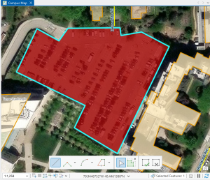
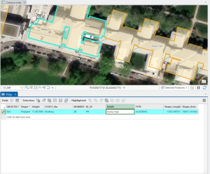
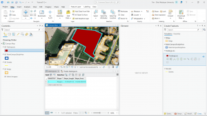
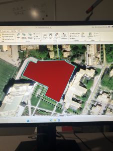
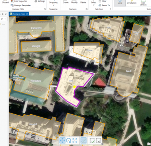
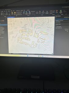
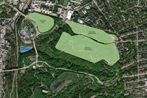
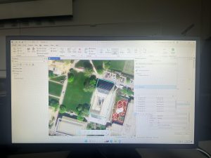
Figure 7.1 Drawing a polygon for the parking lot.
Creating polygons and using the Trace tool were my favorite parts of this chapter! Honestly, making polygons was easier than I was originally expecting. From the readings earlier in this course, I thought I was going to have to input geographic coordinates to put polygons into the correct spot. I learned that ArcGIS is much kinder and allows you to simply drag and rotate polygons. It’s also very helpful to have a matching basemap or base layers to which you can size your polygons.
Also, I was pleasantly surprised by the capabilities of the Smoothing tool. Once again, I thought there was going to be some sort of complicated algorithm I would have to go through to get a smooth shape, but it’s thankfully just another tool! (I’m sure that the computer performs complicated steps, but I am grateful that I don’t have to do them myself.)
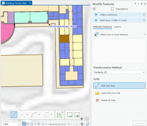
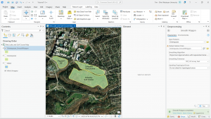
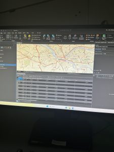
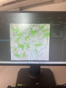
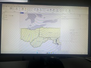
Figure 7.2: Transforming the SpacePlan layer onto the StudyBldgs layer.
It took me a few tries to get this right because I attempted to complete this step before looking at the reference photo in the tutorial. At first, I tried drawing an outline around the SpacePlan layer…which definitely did not work. Then, I tried transforming every single vertex, which was unnecessary. (That attempt is shown in the picture above.)
Chapter 8:
This chapter, focused on geocoding, was pretty short. However, there was still a wealth of important techniques and information within! Something that sounded super interesting to me in the beginning of the chapter was the use of Soundex keys to match attribute names (ex. streets) that are not spelled correctly. It seems like a really neat way to code and simplify language. The step I struggled with the most in this chapter was rematching attendee data. For whatever reason, when I tried to click on an individual location, I struggled to find the Match button and successfully rematch the addresses.
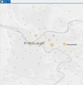
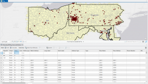
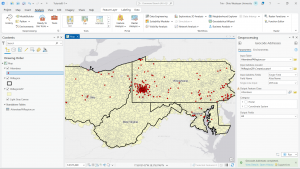
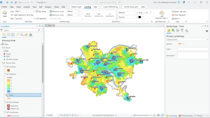
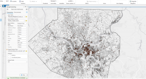
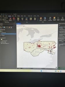
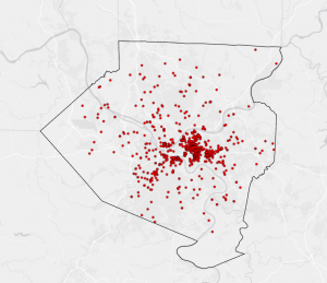
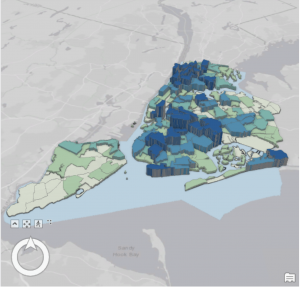
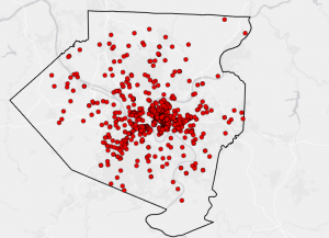
Figure 8.1 Distribution of Attendees using Collect Events tool.
I liked using the Collect Events tool. Being able to turn individual events within certain tracts into collective graduated symbols is a really helpful way to look at the data differently! The concept of match scores is also pretty neat. It’s proof that though the computer is faster at computing than humans, it’s not necessarily smarter. Though the computer does make conjectures and assumptions looking at local context in the data, it doesn’t have the natural reasoning or critical thinking of humans. So yes, mistakes (when inputting addresses, for example) are made by humans in the first place, but then humans go back in after the computer has done its best and apply personal knowledge and community context clues to fill in the gaps.
Chapter 9:
This chapter focused on applying advanced GIS technologies, but thankfully, I found it pretty easy. Tutorial 9-1 introduces the concept of buffers, which I recall reading about in the other text. I find the concept of mapping with buffers really useful and interesting! Buffers are great for determining if objects fall within a certain radius, which is particularly important in fields like public health when determining who may or may not have access to a particular service or facility.
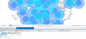
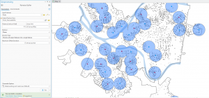
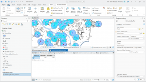
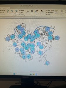
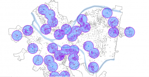
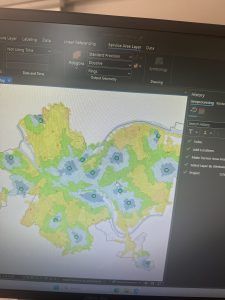
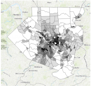
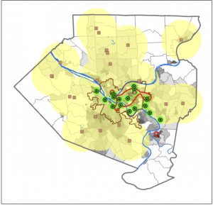
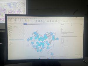
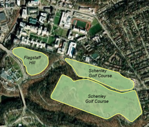
Figure 9.1: 0.5- and 1-mile buffers around public pools in Allegheny County, Pittsburgh.
There are 42, 548 youths in the city of Pittsburgh within 1 mile of a pool, which means 87% of youths in Pittsburgh have good accessibility to a pool. (There are 48,903 total youths in Pittsburgh.) In Pittsburgh, 10,718 youth have excellent access to a pool, 20,448 have good access, and 16,264 have fair or poor access. This corresponds to percentages of 22%, 42%, and 33%, respectively. Considering that more youths in Pittsburgh have fair or poor pool access than those with excellent pool access, changes should be made to ensure that more pools can be open for these kids. (Or alternatively, some areas with high pool density can close and those resources can be reallocated to open a pool in an area where it might be the only one.
In Tutorial 9-5, for whatever reason, some of the Cluster IDs were numbered differently, so I had to pay attention while relabeling the features to ensure they matched the data correctly.
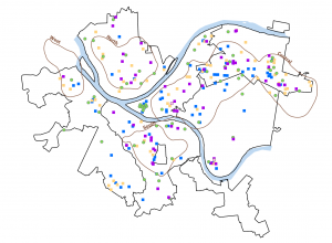
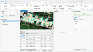
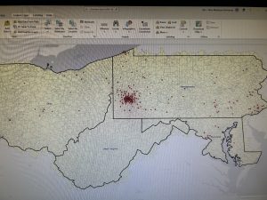
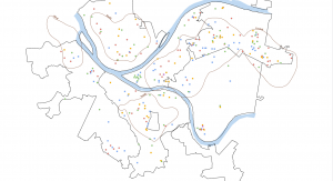
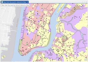
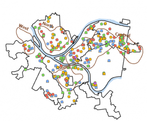
Figure 9.2 Serious Violent Crimes by Age and Gender
The square shapes correspond to young age groups that committed crimes. The pink and purple shapes are females, and the yellow, green, and blue shapes are males. If I were to take this analysis further, I could impose these features on a streets basemap to determine where they are occurring in terms of area development, or I could create a graduated colors map measuring income to see if more crimes are being committed in lower income areas.
All of the tutorials are done…hooray! I just want to give a shoutout to the geoprocessing toolbox…absolutely clutch! I would get so excited every time I saw that I could just plug in my inputs and outputs, units of measurement, and queries. Literal lifesaver. 5 stars.