Hi all, my name is Luke Miller. I am currently a junior majoring in environmental science with a minor in Spanish, and I also play lacrosse.
From the syllabus quiz and reading, I learned that the uses of GIS are vast and varied, being used for environmental, geological, economic, and even medical purposes. Along with this, GIS does not have its own fixed and secure identity, as the user determines its value and how they choose to use it, even within specific fields. For example, a marine biologist might use GIS for completely different reasons than a wildlife biologist. Another variance in the uses of GIS is that it deals with both the “why?” and “how?”, and can be used in different ways based on what the user seeks to answer or find. I enjoyed reading about the first use of GIS, which was to optimize the construction of a highway in a way that would minimally interfere with the environment, which made me wonder what percentage of highways in the US were built using GIS, as I find many of them to be inconvenient. Another concept I learned about was that spatial analysis is different from mapping, as it extracts more data from preexisting data, whereas mapping is just a presentation of existing data. I was also intrigued by the idea that people “reason” using imagery and are able to better understand spatial analysis using imagery. It is for this reason that GIS has become increasingly popular over the years, in that its applications make complex relationships easier to understand and visualize. Finally, I found Bruno Latour’s concept to be interesting in that scientific knowledge and technology must first be disputed to become legitimate. Once they are legitimized, they are then assumed to always be true. This is true with GIS, in that because it has become a legitimized technology, no one questions the validity of its findings, which is both a good and bad thing.
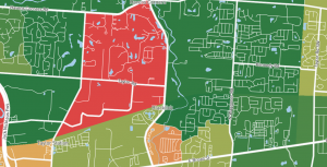
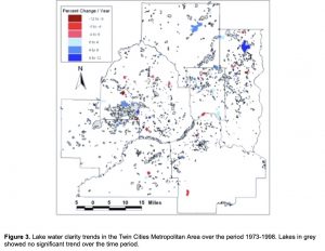
I found the application of GIS to assess the water quality of lakes in my home state of Minnesota to be interesting. In a 2002 study, researchers took existing maps of lakes over a 25-year period and used GIS to correlate them with information about the surrounding areas, such as pollution, to determine the most prevalent causes of water pollution in that specific area.
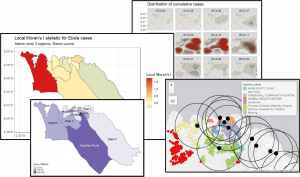
Another use of GIS I found to be interesting was a study conducted in 2009 in Indiana. This study investigated the prevalence of ticks, which are the main cause of Lyme disease, found on deer harvested from 2005-2007. All deer in this study were entered into a GIS database to find where deer ticks were most prevalent.
Sources
Brezonik, P. L., Kloiber, S. M., Olmanson, L. G., & Bauer, M. E. (2002, May). Satellite and GIS Tools to Assess Lake Quality. Water Resources Center; The University of Minnesota. https://citeseerx.ist.psu.edu/document?repid=rep1&type=pdf&doi=7c6ca4d3d77ef0b0417e3f8304f1e66427809323
Keefe, L. M., Moro, M. H., Vinasco, J., Hill, C., Wu, C. C., & Raizman, E. A. (2009). The Use of Harvested White-Tailed Deer (Odocoileus virginianus) and Geographic Information System (GIS) Methods to Characterize Distribution and Locate Spatial Clusters ofBorrelia burgdorferiand Its VectorIxodes scapularisin Indiana. Vector-Borne and Zoonotic Diseases, 9(6), 671–680. https://doi.org/10.1089/vbz.2008.0162