Lydia – Geography 291: Geospatial Analysis with Desktop GIS

I could not do any of the chapter 6 work because of the issues I had with 6a. Here are the things I tried though:
- I completed the steps of the entirety of 6a.
- I first of all used the file I originally downloaded and while the Trees database showed up, nothing would show up, even when I changed the symbology, which led me to discover that there was nothing in the attribute table at all.
- Then, Krygier suggested I download the file onto an external hard drive, so I did that, but the Trees database did not show up at all.
- I then was told that I needed to unzip the new file, which is why the database wasn’t showing up at all, so I unzipped the file.
- Once I unzipped the file, I had the same trouble that I had at first where the database had no data in the attribute table, so I published and skipped the rest.

Chapter 7

Chapter 8

Chapter 9

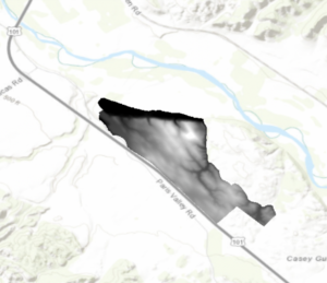
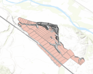
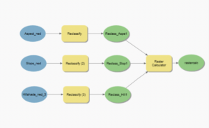
No part of the property is in complete shadow.
Three or maybe four planting sites have relatively low slope topology.
None of the planting sites are in shadow at 2:00 p.m.
The planting site that is closest to El Camino Rd is the best site to plant a new vineyard.

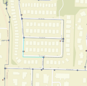
Chapter 10

I had a lot of trouble with 10c, particularly with the titles, but the rest worked fine, so here is what I was able to do.

Luna – Week 4

Posted onFebruary 10, 2023AuthorLydia1 Comment

Getting To Know ArcGIS

Chapter 1 Question Answers and Screenshots
- There were no questions for this chapter, but as a whole, I thought using the website was an approachable way to introduce the basic functions.
Chapter 2 Question Answers and Screenshots
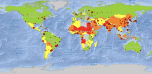
- PM concentrations are highest in Africa.
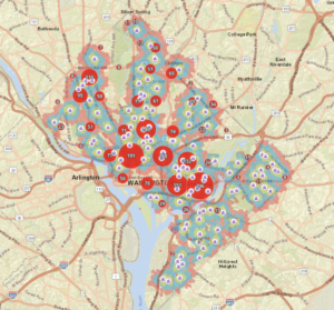
- I used my search bar to restore the Contents pane and find a geoprocessing tool.
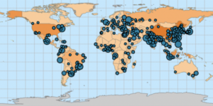
- Shanghai has the largest population.
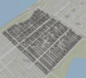
- The height of the tallest building is 339 ft.
Chapter 3 Question Answers and Screenshots
- The field name that indicates state is STATE_NAME and there are 10,575 residents between the ages of 22 and 29 years in Wayne County.
- 7 years are represented by the table.
- Obesity was more common in lower income cities in 2010.
- There are four food deserts in Knox County.
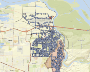
Chapter 4 Question Answers and Screenshots
- The selected line has 4 vertices.
- Shaper_Area decreased.
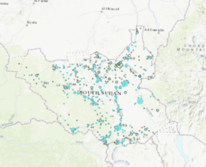
Chapter 5 Question Answers and Screenshots
- I can name the types of conflict events.
- There were 14,211 fatalities in South Sudan between 2010 and 2018.
- There were 71 fatalities in Rwanda between 2010 and 2018.
- There were 41 violence against civilians events in Rwanda and 12 of those were fatal.
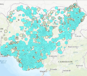
- Summary Statistics and Select are combined in this script.
- 26,323 Nigerian fatalities resulted from violence against civilians from 2010 and 2018.

Luna – Week 3

Posted onJanuary 31, 2023AuthorLydia1 Comment

Chapter 5 of the book talks about mapping “what’s inside.” This is useful because it can help to monitor those occurrences, compare those occurrences with others, and conclude when and how to take action. Areas are defined by drawing boundaries and data can be found in a single area or several and discrete (identifiable) or continuous (seamless) features. Which method is used can be determined by examining what kind of information the user needs from the actual analysis. Some examples of this information may be lists, counts, summaries, or feature views. This chapter discusses three different ways of finding the things inside of an area. The first way is drawing a map that shows the area boundary and the features to see what features are within the boundary. The second way is by specifying the area boundary and features for a summary. The last method is separating the area boundaries and features into different layers, overlaying them, and having the system combine and compare to make summaries. This chapter next discusses how to actually draw the maps, talking about using/mapping locations, lines, discrete areas, and continuous features. Then, it talks about choosing the features that the user wants to use within a boundary, which can be done by the GIS. These results can then be compiled into a report or spreadsheet in many kinds of summaries, including the popular ones of count, frequency, and numeric attributes (sum, mean, median, standard deviation, etc.). Lastly, this chapter talks more about the method of overlaying, discussing the two big categories of using this method with discrete areas and continuous categories. The continuous way uses one of the two methods: vector (compares cross areas) or raster (compares cells). After reading this chapter, I feel more comfortable with the concept of using areas and their contents to draw conclusions and summaries when mapping.

Chapter 6 of the book talks about finding what’s around a feature, which is used to determine the area that is impacted by an event. First, the book explains the importance of specifically defining the analysis, which includes possibly determining distance, travel to and from, cost, and planes (whether it includes earth curvature or not). Next, the user must ask what information is needed from the analysis, which could be a list, count, summary, or distance/cost ranges (may need inclusive rings that show relationships between totals and distances or district bands that compare distances to other attributes). Then, the chapter explains the three ways of discovering what’s nearby, which include straight-line distance (creates a boundary/selects characteristics at a set distance), distance or cost over a network (finds what’s within a manageable distance/cost), and cost over a surface (finds overland travel cost). This chapter then goes very deeply into using straight-line distance, talking about the potential of making and using buffers, just choosing features within a certain distance and the different ways to do/use that, using the GIS to find the distance between features and how to obtain/utilize the results, or creating a distance layer in the program and using it to create specific distance buffers. Next, the chapter talks about measuring over an entire network in the GIS, which means that the system finds all lines in a network within certain parameters. To do this, the user may have to specify the layer for the network, assign segments to centers, set travel specifications, choose surrounding features, and make the final map. Lastly, this chapter talks about finding cost in a geographic surface, which involves specifying cost, personalizing cost distance, collecting the information, summarizing the results, and creating the final map. This chapter was a bit more abstract for me, but I’m sure the concepts will be more clear once we’re using these skills.

Chapter 7 of the book talks about mapping changing conditions or movement in order to predict future happenings, choose a method of action, and interpret the effects of some kind of policy. The first topic in this chapter is defining the analysis, which then goes into the types of change that can be mapped, which include change in location (discrete features and events) and change in character/magnitude (discrete features, data summarized by area, continuous categories, and continuous values). The chapter then moves on to the concept of measuring time, which can be mapped in one of three patterns: a trend (shows increasing/decreasing or direction of movement), before and after (shows impact of event or action), and a cycle (shows patterns in feature behavior). Time mapping can consist of showing the locations at multiple times or the data can be summarized. In both of these methods, the user must choose how many/which dates to include. Then, the user must determine what information they need from the analysis, whether that ends up being how much or how fast the data changed. Next, the chapter talked more about the methods of mapping change which are using a time series (uses snapshots), a tracking map (shows feature movement), or just measurements (shows difference in a characteristic). The book then explains these methods further, talking about ways in which each of them can be used to show change in both location and magnitude/character, methods in constructing the map itself, and how to examine/use the results. Finally this chapter concludes by talking about ways to report the results and methods in summarizing. This chapter was one that felt very straightforward. I found it useful that it showed ways to use each method as well as showcasing the pros and cons of each, which will be helpful when choosing what way to do things.

Luna – Week 2

Posted onJanuary 25, 2023AuthorLydia1 Comment

Chapter 1 of the book really focuses on the basics of GIS. It firstly discusses the chapters of the book and the way that they are ordered so that they teach you to do the basic process that is followed in GIS. Next, this chapter works to make the reader understand geographic features. Firstly, the types of features are covered, including discrete features (features with real locations that can be specified), continuous phenomena (occurrences that are experienced and measured everywhere using locations with boundaries or random sample points), and features summarized by area (the measurement of the features within certain boundaries that apply to the whole area rather than a specific place). Then, the chapter talks about methods of modeling features. The first of these methods is the vector model, where each feature has its own table row and the shapes of these features are shown by their coordinate location on the graph. In the raster model, which is the second method, features are shown using cells in space. This part of the chapter also talks about map projections (shows locations of a spherical globe on a flat map) and coordinate systems (specify units that are for finding the features in a flat space). The next section discusses geographic attributes and the types of them, which are the continuous ones, including categories (groups) and ranks (orders), and the noncontinuous ones, including counts (number of features on a map), amounts (measurable feature quantities), and ratios (relationships between quantities). Finally, the last section covers the use of data tables, talking about the operations used including selecting, calculating, and summarizing. This chapter, as a whole, did a very good job of showing what GIS is all about and why it is needed using the types of features that it is used for to show its need.

Chapter 2 of the book is more about mapping and what goes into that process. The first part of the chapter says that it is important to map things because maps can either show what places meet the requirements, where the most action is needed, or why things are happening. The second part talks about how to decide what to map, firstly saying that the user initially needs to ask what information is actually needed when the analysis is done and how the map will be used. The third part covers how to prepare the data being used, which requires assigning geographic coordinates and category values. The next section of the chapter talks about actually making the map that all of this will be on. This part talks about mapping features of the same type using the same kind of symbol, GIS’s purpose of storing the location as points or shapes, and mapping using feature subsets, which is said to be more common than using individual locations. Next, the books discussed mapping categories, saying that GIS works to store category values for each of the features in the data, making it able to display certain features based on their type. Symbols or colors can be used to differentiate these groupings but the book instructs the user to be careful because too many colors or symbols can make things confusing. This section also suggests that the user use reference features, or landmarks to make it more meaningful to people. Finally, the last section of this chapter discusses interpreting patterns that can be seen in maps. This chapter is a very digestible introduction to actually being able to do things in GIS. While the first chapter talked a lot about the history and use, this one left me feeling better prepared for using the program.

Chapter 3 is about mapping the most and least, which is said to be useful because it can assist in finding data points that fit in the needed criteria. In order to do this, the values need to have quantities assigned to them, which can be assigned to discrete features, continuous phenomena, or information summarized by area. The next section of this chapter covers the quantities and actually understanding them by more deeply explaining counts, amounts, ratios, and ranks. After this, the book talks about grouping the quantities together into classes, which is said to be particularly useful when it comes to some kind of public presentation because it allows easy comparisons. The text points out that while charting individual values is more accurate as a whole while also allowing raw data patterns to be seen, it is much more effort. Classes, on the other hand require less effort and can be either made manually (when using specific criteria or specific comparisons) or by a standard classification scheme (when grouping to search for patterns). The classification schemes, that are chosen by determining how data is distributed, include natural breaks (finds inherent patterns in data to separate based on those), quantile (each class has the same number of features), equal interval (each class has the same data range), and standard deviation (classes are defined by their distance from the average). This part also talks about outliers and deciding how many classes to use. Lastly, this chapter teaches the reader how to actually make a map using graduated symbols or colors, charts, contours, and 3D views, while also explaining how to effectively use each of those components. This chapter really helped me understand the different ways to interpret data when it comes to GIS, which is different from the past two chapters and will help me when making maps.

Chapter 4 covers the topic of mapping density, and therefore concentrations, of features, which is helpful in recognizing patterns. This chapter talks about how to decide what to include in the map, which requires knowing what kind of data is being used and what kind of values need to be included, meaning either locations or features of the locations. There are two ways to map density. The first uses features summarized by area and should be used when there is previously summarized data or defined borders while the second includes making a density surface using the GIS and should be used when looking for the concentration in features. Next, this chapter talks about how to map density in defined areas, which can be done by finding a density value for those areas, making a map with dot density, or asking the GIS to summarize the features. Lastly, this chapter explains how to create a density surface. The GIS defines an area based on the radius that the user specifically determines, counts the number of those features in that circle, and divides that counted value by the area of the circle. The way that the GIS determines this relies on multiple factors, including cell size (the coarseness of the patterns), search radius, calculation method (either simple or weighted) and units. The density surface is then displayed with contour lines, which connect equal density points on that generated surface, or graduated colors, which can either be used by creating custom ranges or commonly used classification schemes. Finally, the user must view and interpret the result, which mainly involves finding patterns that depend on what kind of density surface was made. This chapter was a bit more confusing for me, but still helped me to further my understanding in the topic of GIS, especially once I get to do it for myself.

Luna – Week 1

Posted onJanuary 19, 2023January 19, 2023AuthorLydia1 Comment

Hello! My name is Lydia Luna. I am a sophomore Zoology/Environmental Science double major from Mount Vernon Ohio. On our campus, I am involved in Greek Life, Panhellenic Council, Campus Programming Board, and the Admissions Office.

As I read Schuurman Chapter 1, I initially found it very exciting (or as exciting as a book like this can be) that the author of this text is directly aiming to instruct not only technically-skilled individuals but also those (like myself) that may not be overly familiar with this kind of program. I also found it interesting that the author explicitly talked about all of the different roles that GIS can play in society, which furthers the idea that GIS and this text specifically are not only for the people that you would automatically think about. I also really enjoy when someone that is teaching a topic can not only see why their work is important, but also the flaws in it. Reading the author addressing the flaws in these programs makes it seem like when I inevitably get frustrated in the process of learning how to use them, I’m not alone, which is an oddly comforting feeling. The explanation of the two components of GIS was new to me, with there being a “systems” side of things and a “science” side of things. It was very interesting to learn about how GIS can mean different things to different people, even outside of the different core uses. On top of that though, the authors also discuss the overlap in the two, which revolves around the concept of space. Once the space is officially called data, then it goes into the two components, whether to be collected or classified. It shows that while all of this kind of stuff can be very different and can be used for many different purposes, it all comes from the same core data. As a whole, this chapter just made GIS seem much more approachable and useful, no matter what career field I choose to go into.

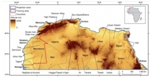
One of the applications of GIS that I looked into was in the realm of conservation, as I am interested in the use of environmental science in the zoology world. In the article I found, GIS was used to observe the changes in the environment in Northern Africa in order to explain the changes in biodiversity there. I also looked into the applications of GIS in water resources, which gave me an article about how the program can be used to model the way that water management would work in different locations before actually installing different methods.

Sources:

Brito, J.C., Biogeography and conservation of taxa from remote regions: An application of ecological-niche based models and GIS to North-American canids. Biological Conservation 142, 3020-3029 (2009). https://doi.org/10.1016/j.biocon.2009.08.001
Tsihrintzis, V.A., Hamid, R. & Fuentes, H.R. Use of Geographic Information Systems (GIS) in water resources: A review. Water Resour Manage 10, 251–277 (1996). https://doi.org/10.1007/BF00508896