Geography 291: Geospatial Analysis with Desktop GIS

Chapter 4 (Mapping Density):

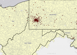
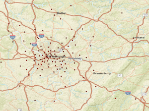
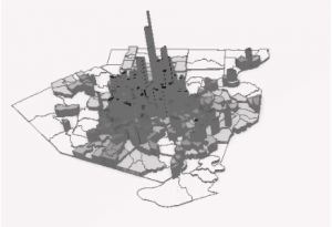
Density maps give a clearer distribution array than simply mapping features.

Two types of density mapping: based on features summarized by defined area or by creating a density surface

Defined area: Ex( Using a dot map to represent density of individual locations)

• Use if data already summarized by area or in lines/points easily summarized by area
• Easy, but doesn’t pinpoint exact densities

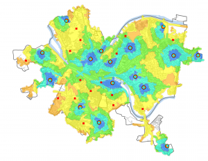
Density Surface: Ex( Raster layer with each cell being assigned a density value such as per square mile)

• Use if given individual locations, points, or lines
• more precise view of density, but is more difficult

pop_density = total_pop / (area/27878400)

27878400 square feet in a square mile

Dot density map seems to be a combination of defined area and density surface.

It is possible to map defined areas using individual features, but you have to make sure it meets your criteria.

When GIS runs the program to create density surface it creates a neighborhood or area around each cell that creates a smooth transition from cell to cell.

How to find the right cell size:

1. Convert density units to cell units
2. Divide by the number of cells
3. Take the square root to get the cell size (one side)

Finding the right cell size is just finding the sweet spot between not using too much processing power while still showing the detail of patterns.

It is possible to map density surface with data summarized by defined area. You can use census tract centroids for each cell to create a smoothed surface.

It is possible to use the four different classification schemes to achieve different outcomes.

Often higher densities are shown using darker colors, but using lighter colors could draw the reader’s eyes to the area more effectively.

Chapter 5 (Finding what’s inside):

In order to map what’s inside you need to define your area of study and combine that with features to create summary data.

Single area:

Analyzing activity or summary information in that area

• A service area around a central facility
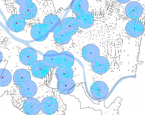
• A buffer that defines a distance around some feature
• An administrative or natural boundary (parcel of land or watershed)
• Manually drawn area (proposed sales territory)
• Results of a previous model (floodplain modeled in GIS)
• Combination of several areas treating them as one

Multiple Areas:

• Contiguous (such as zip codes or water sheds)
• Disjunct (state parks)

Discrete features are unique, identifiable features. Continuous features represent seamless geographic phenomena.

When using a list or count of features you should include those features that are partially within the boundaries of the mapped area.

Three ways of finding what’s inside:

Drawing areas and features:

• Create a map showing the boundaries of areas and the features to see if features are inside the areas. All you need is a dataset containing the boundary of the area/s and a dataset containing the feature/s.

Selecting features inside the area:

• Specify the area and the layer containing the features, then GIS selects a subset of the features inside the area. Good for getting a list or summary of features inside an area. Need a dataset containing the areas and one with features.

Overlaying the areas and features:

• GIS combines the area and the features to create a layer with both attributes to compare them. Good for calculating summary statistics and finding which features are in each of several areas, or finding out how much of something is in one or more areas.
• Need data with areas and data with features (including attributes you want summarized)

Shade outer area to emphasize features and fill outer area with translucent color to emphasize outer area when mapping discrete areas.

If a feature falls within two or more areas, the GIS splits the feature where it crosses the area boundary. Most any types of maps can be overlayed for comparison.

Chapter6 (Finding what’s nearby):

Mapping what’s nearby can be used to find out what’s happening within a set distance of a feature.

Distance can be measured in distance or travel cost.

Three methods:

• Straight-line Distance
  good for creating a boundary or selecting features a set distance away from a feature. Layer containing main feature and surrounding features.
• Distance or cost over a network
  Good for finding what’s within a certain travel distance/ travel price over a fixed network. Need locations of source features, a network layer, and a layer containing surrounding feature (usually)
• Cost over a surface
  Good for calculating overland travel cost. Need layer containing source features and a raster layer with the cost surface.

Choosing a method:

• straight-line when defining area or want a quick estimate of travel range
• cost or distance over network when measuring travel over a fixed infrastructure network
• cost over a surface when measuring overland travel

When analyzing features within an area color-coding can be used to draw attention to different categories of features.

When creating a distance surface you can set a maximum distance for which GIS will only calculate to that point.

Cost in a cost over surface map can be time, money (such as cost to develop an area), or effort expended. For example a deer might expend less energy moving through open forest than through thick brush.

Is an elevation/ topography map a version o a cost over surface map?

A lot can be done with a cost over surface map. No maximum can be set, or a maximum can be set, or the area outside a certain limit can be selected.

When using more than six or seven ranges, you can use two or three hues to help distinguish the ranges.

Chapter 4
Two ways to map density: by defined areas or by density surface.

defined areas: you can show and calculate density for the defined area. You can use a dot map.

density surface: created in GIS raster layers. Simple calculations are not as easy to read as weighted calculation in terms of rings. You can use graduated colors or contours to map density surfaces. Be aware of how many class you use, between 3-15 is the sweet spot, more or less gets confusing and loses data. Also note the colors you choose for the gradient and what appeals to the eye more (dark or light color gradient indicates high density).

Be cautious of how much info we need or don’t need, it’s a fine line between too much and too little info to not lose the obvious patterns in densities.
I remember calculating cell size conversions in remote sensing, it took such a long time. I think I left for lunch, used the restroom, got Rowley coffee and it still wasn’t done. I think I was converting points to tangible pixels with units but it’s crazy how much power and time it takes for these things sometimes.

This chapter was pretty short and covered a lot of things I knew how to do technically, but gave me more info on the use and reason behind these techniques. I liked comparing the dot and contour maps, I think it would be cool to do something with those in a project.

Chapter 5
to find out what’s inside, first build you area of study, and if its one or many.
I recall searching for feature attributes in remote sensing to narrow down a price range for potential house buyers. I also remember trying to import a boundary layer (shapefile) of Brazil and it kept not working. The datums were the same but it was not wanting to place itself properly. It took me 2-3 days to figure out how to do it.

Drawing areas/features: find whether features are in area or not. good for single area.
Selecting features in area: get a list of features in area, good for single area.
Overlaying areas/features: which features are in which areas and how many/how much in that area. good for multiple areas.

Most common summaries: count and frequency.
count: the total number of features inside the area, such as the number of businesses in a neighborhood.
frequency: the number of features with a given value, or within a range of values, inside the area, displayed as a table.

These slivers are very annoying. I remember making data points on a top layer that was slivered and when I flushed it out those data points were nulled because they didn’t fall in the area. I had to go back and move the points in just a hair to get them to be present.

The vector method provides a more precise measure of areal extent but requires more processing and postprocessing to remove slivers and to calculate the amount of each category in each area.

when choosing overlay to remove slivers: the raster method is more efficient because it automatically calculates the areal extent for you, but it can be less accurate, depending on the cell size you use. also prevents the problem of slivers. It is often faster because the computation that the GIS must do is simpler.
single area with one category: bar chart, or pie graph; multiple areas with one category: bar chart; multiple areas with multiple categories: histogram, cluster, or stacked bar chart, with few areas/categories you can use pie chart too

Chapter 6

I didn’t consider time or effort a cost in distance before this chapter.

Planar: calculating distance assuming the surface of the earth is flat

geodesic: taking into account the curvature of the earth when calculating distance

Inclusive bands: tells you the total number within bands as distance increases

distinct bands: lets you compare distance to other characteristics like how much someone 1000m away spends on groceries compared to 2000m.

I like the chapter setups where it introduces a concept, tells you its pros and cons, and also tells you how GIS does it as a function/what you need to do it, etc. Its helpful to have consistency. 

These few chapters have covered a lot of what was in our exercises for remote sensing. I had to do parcel selection within a given boundary to find homes for homebuyers that met their specifications.  I was reminded of this when it discussed selection within boundaries. I’m glad that a lot this is getting explained now. I would get pretty confused doing raster calculator calculations and not understanding what the numbers and symbols I entered meant. It is plugging in data into the calculator as a word problem too, the worst kind of math.

The spider diagram is cool, I like it. The graduated symbols map seems harder to read, the graduation of triangle size is hard to distinguish (for me)

The calculation of these distance seems like a really useful tool. I have worked with this concept a little bit but not to the extent that they went into in this chapter. I learned more about what Arc is doing behind the scenes in my random clicking and it makes things more comprehensive for me. I am more aware of why I’m doing something as opposed to just following directions to get it done.

 

Ch.1

Not everyone can just go into GIS, but you need to understand the proper tools and structure for your intended analysis. I think it is interesting how a lot of GIS users become advanced analysts, so that is another possible career path.

GIS Analysis: a process for observing geographic patterns in a set of data and at relationships between different features.

It is important that you understand your data and be able to find the proper way to develop it.

Important Steps to GIS Analysis

Frame the question > Understand your data > Choose a method > Process the data > Look at the results > Understanding geographic features

Geographic features are discrete, continuous phenomena, or summarized areas.

Discrete features: are discrete locations and lines, the actual location can be pinpointed. At any given spot, the feature is either present or not.

Continuous Phenomena: examples are precipitation or temperature and can be found or measured anywhere. You can determine a value at any given location. 

It is important to note that continuous data often starts out as a series of sample points, either regularly spaced or irregularly spaced.

Example of regular spaced: sampled elevation data

Example of irregularly spaced: weather stations

Interpolation: Where GIS can use sample points to assign values to the area between points.

Sometimes non continuous data can be treated as continuous in order to create maps showing how a quantity varies across the place. Continuous data can also be represented by areas enclosed by boundaries-if everything inside the boundary is the same type- such as a type of soil or vegetation. 

Important Note: “If the features aren’t tagged with the codes for the areas by which you want to summarize them, the GIS lets you overlay the areas with the features to identify which ones lie within each area and to tag them with the appropriate code”.

Vector and raster are the two ways geographic features can be shown in GIS. It is important to use the right size when dealing with these models. Continuous categories are represented by vector or raster models. Continuous numeric values use raster models only.

Geographic features have specific attributes that go with them.

Examples: categories, ranks, counts, amounts, ratios

Categories are groups of similar things. (not continuous)

Ranks put features in order, from high to low. (not continuous)

Counts and amounts show you total numbers. (are continuous)

Ratios show you the relationship between two quantities and are created by dividing one quantity by another for each feature. (are continuous)

Important: working with tables that contain the attribute values and summary stats is a vital part of GIS analysis. Three common operations you perform on features and values within tables are SELECTING, CALCULATING, and SUMMARIZING.

Select attribute= value

Select Landuse= com

Select Landuse= com and acres > 2

CH.2

A lot of people use maps, use them to see where, or what, an individual feature is. Patterns are often seen. Individual features vs distribution of features. 

GIS can tell police officers where to assign patrols based on crimes that occur.

Step 1: Need to decide what to map

• Decide what features to display

Step 2: What info do you need from the analysis?

• Might need to know where features are or are not? The question. Patterns.

Step 3: How will you use the map?

• Appropriate audience
• Make sure issue is being addressed
• Make sure to add just  the right amount of info(no unnecessary details)

Step 4: Preparing your data

• Make sure the features you’re mapping have geographic coordinates assigned and, optionally, have a category attribute with a value for each feature before mapping

Step 5: Assigning geographic coordinates

• Each feature needs a location in geographic coordinates

Step 6: Assigning category values

• Each feature must have a code that identifies its type, when your map FEATURES BY TYPE, example is whether a crime is burglary or assault
• In some cases, a single code indicates both the major type and subtype

Step 7: Making your map(finally!)

• Tell GIS which features you want to display and what symbols to use to draw them
• You can do this by creating a layer for either single type or categories

Mapping a single type

• Must draw all features using the same symbol

You can map all features in a data layer or a subset you’ve selected based on a category value.

Using a subset could reveal patterns that aren’t always apparent.

Step 8: Mapping by category

• You can understand how a place functions when mapping by a category(roads like freeway and highway)

How many categories? Want to display no more than seven categories and grouping them could make it easier to understand/distinguish. Example: 18 categories grouped into 5

Just know that GIS is very complicated, complex and delicate

You can group categories in several different ways.

1. Assign a general code to each record in the database
2. Create a linked table to match detailed codes with general codes
3. Assign categories on the fly by specifying symbols

Choosing symbols: make sure the symbols you choose are chosen carefully(combination of color and shape)

The map you create will be more understandable if you display recognizable symbols. Include a map reference if you think there is a chance that people won’t get it.

Step 9: Analyzing geographic patterns

• Pretty self explanatory(look for patterns)

CH.3

Why map the most and least?

• Lets you compare places based on quantities, so you can see which places meet your criteria

In order to do this… your map features must be based on quantity associated with each.

Mapping features based on quantities adds an additional level of info beyond simply mapping the locations of features. 

To map?

• Need to know the type of feature
• Know the purpose of your map

You can map quantities associated with discrete features, continuous phenomena, or data summarized by the area.

Locations can be dotes

Lines can be rivers

You might want to present your map in a specific way, but must explore the data first.

Knowing quantities(counts and amounts), will be important or could be when presenting your map. You can map counts and amounts for discrete figures. 

• Might need to summarize by area’

Might need to show ratios to get your point across…averages are good and so are proportions.

Proportions are often presented ias percentages. Densities show you where features are concentrated. 

Ranks: poor-fair-good-excellent or 1-8

Once you’ve determined the type of quantities, need to decide how to best represent them on the map.

Might need to make trade-offs when doing this.

Mapping individual values could be very important in order to present a more accurate picture.

You will need to keep in mind classes and how to create them manually.

The four most common schemes are natural breaks, quantile, equal interval, and standard deviation. GIS can compare these different classification schemes.

Good: mapping data values that are not evenly distributed

Bad: difficult to compare the map with other maps.

There are pros and cons to each different common scheme.

You might need to deal with outliers in your data, so know how to deal with them.

Note: might have to decide how many classes to include and make them easier to read using GIS

Towards the end of chapter 3. Talks more into detail about features and details about maps.

Might need to use charts, contour lines to map data. 

GIS can create 3D perspective views! How awesome!

1.      GIS Analysis can be defined as looking for geographic patterns in data that is found and is also used at looking at patterns in relationships between features. The process can be described in a few short steps. First, frame the question, understand the data, choose a method for how you will get said data, process the data, and finally look at the results. There’s different types of geographic features and it’s important to understand when dealing with mapping. 

• Discrete features- I think they gave an unclear definition for this but I got another definition from Esri. It’s defined as discontinuous but has very defined features. 
• Continuous Phenomena- An example of this is precipitation and it can be measured anywhere
• Summarized by area- Represents the density of singular features within a certain boundary or area. 

When learning how to map, it’s important to understand the geographic features and their attributes. 

• Categories- Groups of things that are alike. Example, categorize roads as highways, alleys, or etc. 
• Ranks- Puts things in order specifically from high to low. To put this into context of geographical measures, it may be hard to find a direct measure. An example they gave is assigning soil as all the same suitability for a plant. 
• Counts and Amounts are grouped into the same category and are both defined as it shows you total numbers. They are then specifically defined. A count can be defined as the actual number of features on a map. An amount is any measurable quantity that is associated with a feature. 
• Ratios- the relationship between two quantities and are created by division. One quantity is divided by another for each feature. It’s like taking an average. 

You also have to work with date tables when learning GIS. There’s a lot to GIS. Using data tables you have to learn selecting, calculating, and summarizing. 

2.       Chapter two is all about mapping. You have to decide what to map, obviously, before you start going crazy. Much like writing a book or article, your focus has to be right and you have to make sure you’re reaching your target audience. The mapping also has to be well organized and relatively easy to follow just like a book, it has to make sense. Kind of off topic but I’ve seen people on TikTok trace a pile of Rice to make a country and they make different features on the map and I thought that was really cool. Anyway, to make a proper map you need to make sure the features you map have geographic coordinates assigned. This means including the latitude and longitude of each mark. To make the map easier to read, you need symbols for different attributes. This makes it easier to see patterns. GIS does the work for you when trying to map something out. Its job is to use the coordinates to draw the attributes or features using the symbol of your choice. You can layer data and then select a specific thing you want to see by itself instead of seeing every feature together. This is very useful when you want to find specific patterns. This can be used in Apple Maps when you’re looking for close attractions but only want to see restaurants. GIS is widely used around the world, but I think not everybody knows the proper name for geographic information systems. When mapping categories, they suggest limiting it to 7. This is because the map could potentially become hard and confusing to look at. The scale matters when mapping these categories because the said features are spread out, then you would be able to map more categories without making it hard to understand. 

3.      This chapter is called the “Most and Least”. They phrase it as mapping the most and the least places lets us compare things based on the quantity. I thought this was a bit weird at first because I think mapping everything would be the most accurate. Maybe it would be the most accurate but mapping everything makes it harder to understand and could make the map convoluted. This chapter talks about how you have to keep one focus on your map and keep the intended audience in mind. I already stated this in the above chapter and said how making a map is kind of like writing an article. You have to keep the map purpose from drifting off. This chapter seems like a review. Quantities can be counts or amounts and knowing the difference will help you best pick which one to use for a map.  

     A new idea they introduce is density. When densities show in a map it shows where those features are most concentrated. The chapter starts going into data like statistics. I know this is important to GIS but I hate math. Matter of fact, I took stats during COVID so I actually learned nothing. What I know about stats is that I hate everything about it including standard deviation. The easy thing to understand about stats is that some data may have outliers. This means that there will be points that lie way outside of the average points. This could then skew the data either left or right. There’s different ways to label and create a map including graduate symbols, colors, contours, charts, and 3D viewing. Graduated symbols show a range of values. Charts show categories and quantities. These are for discrete areas. You can use pie charts and bar graphs to show data as well but I think we all know that. 

Chapter 1: Introducing GIS Analysis

Some comments, notes, and questions I had while reading this chapter were plentiful. It was interesting to find out that spatial analysis is working to bring attention to real-world problems and issues people face. GIS is growing rapidly and we are finding more and more uses for its capabilities. GIS analysis is using models of the real world and looking at the geographical patterns. There are 3 types of geographical features: discrete, continuous phenomena, or summarized by area. Discrete locations and lines are actual spots found and can be easily read line buildings or bodies of water. Continuous phenomena are going to span the whole map you make because it shows weather patterns like rainfall or temperature. Interpolation is when GIS gives values to points irregularly or regularly spaced on a map. Geographical features summarized by area could be the number of households in each county, or business zip code. Reading about the two types of GIS models vector and raster I am a little confused. A vector model is a map that shows a point and is labeled using x and y coordinates mainly used to show small details. The raster model is for larger spaces that need to be analyzed and is not good if looking for precise measurements. I thought it was interesting to find out that map projects get distorted because of the curvature of the earth. So when looking at a large section of Earth it will relatively not be 100% accurate. After reading about ranks and counts and amounts for features that are mapped it gives me an idea why different levels are color-coded and categorized for their particular purpose. How will summarizing the values of a large population help us to find an average? Will data tables help to sort out ranks for a map that needs to be created? 

 

Chapter 2: Mapping Where Things Are

Why map where things are? To see patterns that may need another perspective besides being in a table or literature. What is the difference between distribution features and individual features? Distribution features are patterns and many professionals use GIS to target areas they are in need of their assistance. Deciding what to map? Is a process since you want a map to be easily read and understood and to correctly convey information to readers. Learning how to create features to be layered over other features to display different years or a pattern of change. Being detailed on either category or doing a broad overview to minimize distractions for the intended audience. Preparing data needs to be organized before starting a map and to have all features with a location. How will geographic coordinates be assigned to the GIS database? Will we be learning how to code features or will the software we use already be coded? It was neat to find out that we just told the GIS what features and symbols we wanted to be shown. Mapping a single type may or may not be able to show patterns but for a single type, all the same symbols will be used. What is the main idea behind GIS? It has many capabilities for setting coordinate pairs and storing the locations, symbols, and streets. Using a subset of features to layer data was neat to show the relationship between two completely different categories. 

 

Chapter 3: Mapping the most and least

To find a place to map you should look for areas with equal quantities of an abundance of species and, or a place with a decline or decrease in species. It’s all about finding information that will be helpful to us in the future. What we need to map is finding patterns with similar values with quantities that should be studied. The features we will be focusing on mapping will be centered around discrete and linear features. The continuous phenomena are areas that cover. When looking at a map or creating one the dark areas will be greater in value from lighter shades. All ranks will be coded in this way so that the more pigmented areas will be darker or have more than light colors. A map that shows the longest salmon runs were categorized and coded on a map and from the pattern it was determined that the counties will longer runs have watersheds. The difference between presenting or doing research with a map will be set up in two separate ways. If presenting a map it will need to be simple to show a pattern and a more generalized view. If doing research on a map it can be detailed and have lots of different features.  Business can be mapped by the number of employees and the size of circles will be used to show employment numbers. For a larger area say the whole state of Ohio using counts and amounts would be the most beneficial and it will be rounded numbers. Block groups vary in size so a rough guess would be sufficient.  Using ratios to show the distribution of features with averages, proportions, and densities. 

Chapter 1: GIS itself is the process of looking at geographical patterns in your data and at the relationship between the features within said data.

Start by framing your question: This can typically start off as a question, and being as specific as possible about the question you are asking will help with deciding the best method to approach it with.  Understanding your data can also aid in making things more clear and narrowing down what method you should use. Finish by looking at your results and deciding if the data is relevant/useful, or if you should use a different approach.

There are multiple kinds of features in GIS: For discrete locations and lines, the actual location can be pinpointed, and the feature is either present or not. Continuous phenomena like precipitation can be found or measured anywhere. Summarized data represent the counts or density of individual features within area boundaries.

Vector and Raster: With the vector model, each feature is a row in a table, and feature shapes are defined by x, and y locations in space. With the raster model, features are represented as a matrix of cells in continuous space.

Types of attribute styles: Categories, ranks, counts, amounts, ratios

The only thing I worry about from this chapter is coming up with my own question. There are so many different topics with so many different subtopics, and the possibilities are so open that it’s almost overwhelming.

Chapter 2: Prepping your data involves ensuring that the features you are mapping have geographic coordinates assigned and have a category attribute with a value for each feature. If you are bringing data from another program or entering it by hand, the features will need to have location information like a street address or latitude-longitude, and GIS will assign the coordinates.

To make your own map, you’ll tell GIS which features you want to display and what symbols to use to draw them. Mapping a single type involves drawing all features with the same symbol, while mapping by category involves using a different symbol for each category. If you use the method with multiple categories, you shouldn’t use more than seven categories, otherwise, you will have to group categories.

Along with symbols, text labels can also be used to help distinguish categories (e.g. OW = Open water)

Chapter 3: This chapter continues to discuss different methods of displaying data, as well as how they should be understood. It seems like the best method for display varies between the project and what its purpose is.

Natural breaks: Data is not evenly distributed

Quartile: Data is evenly distributed

Proportion: part of the whole

Rank: high, medium, low

Density: concentration of data/feature

I found all three chapters helpful in terms of explaining the basics of GIS. There are pictures to illustrate every point that is made, which is super helpful for me, as I have always needed some kind of visual or example to understand any concept.

GIS ch1

 

This first chapter broke down the basics of GIS. What to use it for, how to use it, and which options are best for depicting different types of data. A big part of this chapter was the introduction of vector models and raster models. Vector models are often coordinates and lines that are the summary of data tables. Vector models are especially useful for discrete data which are values more specific than the alternative continuous values. On the other hand, the raster model is more useful for continuous numerical values. Raster models are depicted as cells that can be combined side by side with other cells to show how the data connects or overlaps. Layers are more prominent and used more often in these models. Another key difference between raster and vector models is that raster is more scale sensitive. Distortion can happen in all models and all scales but it is most significant in raster models. To counter this, you can find the appropriate sale from the original scale and the minimum map unit. Between these two models, continuous categorical values can be used and seen in either. This also brings up the continuous phenomena. The continuous phenomena describes how certain analytical values can be found or measured anywhere. 

Another important factor of GIS is layering. This chapter gave some good information on how overlaps can make tags for pieces of information which can then be used for layering. 

Towards the end of the chapter, categories, ranks, counts, and ratios show up. These are all attribute values that are important factors in GIS. Categories are values with a common aspect. Ranks are orders assigned to categories. Counts are total numbers. Ratios show the relationship between two or more categories. Categories and ranks are noncontinuous values because there can be the same value while counts and ratios are continuous values because they are completely unique. 

 

GIS ch2 

 

In this chapter, more of the mapping mechanics were thrown out there. Things such as category classifications, scales, and vector and raster models were revisited along with the addition of the use of subsets, grouping, zooming options, and colors or shapes of a map. From all of these other factors, chapter two explains the change of patterns. Patterns can be much more recognizable when you use a distribution of data instead of more individual sizes for the map. Using subsets can bring more detail to certain categories which could also bring out some unseen patterns. Similarly, zooming in or out can show us new things based on the original map scale like discussed in chapter one. For the sake of clarity, many large scale maps don’t use shapes for location points because with so many points it may be hard to recognize the shapes in clusters. In smaller scale maps, more colors and related categories can be used because there is less area to focus on so it will add detail without subtracting clarity. For this reason it is suggested to use no more than seven categories on large scale maps but if there are more, there is the option of grouping. This sometimes jeopardizes important information for the sake of clarity but can even emphasize already existing patterns that were not as prominent. 

Chapter two made me excited to start thinking about ideas for my own GIS maps. With all of the examples being featured along with the first look into how we will be doing this unfamiliar task, my mind is stirring. A lot of these examples were crime based and from seeing all of them I feel like I have a pretty good basic understanding of crime patterns shown here. This gives me a sort of reference point for how I want anyone viewing maps that I may make to see them. Aiming for clarity along with detail and distinguishable patterns. 

 

GIS ch3

 

Chapter three is about being able to understand what you’re putting in a map and what purpose each feature has. This chapter also mentions these factors from an audience perspective along with an exploratory perspective. Either way, you start with determining certain types of quantities like the previously mentioned ranks, counts, and ratios. This time, there is an addition of averages, proportions, and densities used to present gathered data. Averages are used when there are not a lot of features in one area and a lot in another area and you need to find a connection between the two. Proportion is used to find part of a larger whole or break down a large scale into a smaller scale. Densities are used sizes in an area that have a lot of variety. Another important strand of terms is the ones used for creating classes. Natural breaks, quartile, equal intervals, and standard deviation. Natural breaks are classified by jumps in the raw data and are useful when data is not evenly distributed. Quartiles are classified by similarities in numbers of features (low to high) and are good for data that is evenly spread. Equal intervals are classified with even amounts of highs and lows. It is simple to understand and good for continuous data. Standard deviation is classified by distance from the mean which makes it good for comparing values to an average. 

Other useful pieces of information in this chapter were what to do with outliers depending on the type of map you use and the types of features. Also, the use of raw data is interesting because a lot of times raw data is good to look at for lots of detail, but it does get overwhelming if presented to the audience who may not have as much previous knowledge on the topic represented in the map as whoever collected or used the raw data. 

I found the section providing examples of all the map features and their advantages and disadvantages helpful because it pulled all of the beginning chapters together in a visual way. It also just summarizes a lot of the past chapters so I think I’ll be referring back to those pages later on in this course.

1)

Common uses for geographic analysis: Mapping where things are, Mapping the most and least, Mapping density, Finding what’ s inside, Finding what’s nearby, Mapping change

GIS analysis is a process for looking at geographic patterns in your data and at relationships between features.

Process: Frame the question, Understand your data, Choose a method, process the data, Look at the results.

Geographic features are discrete (the actual location can be pinpointed; at any given spot, the feature is either present or not) , continuous phenomena(blanket the entire area being mapped, but a value can be determined at any given location), or summarized by area (density of a variable within area boundaries,.Data applies to entire area, but not any specific location within it).

Vector Model: Each feature is a row in a table, and feature shapes are defined by x,y locations in space. Analysis involves working with (summarizing) the attributes in the layer’s data table. Better for discrete features and data summarized by area.

Raster Model: Features are represented as a matrix of cells in a continuous space. Analysis occurs by combining the layers to create new layers with new cell values. (must use perfect cell size: too small requires too much storage and takes longer to process, too large will cause detail and information to be lost). Better for continuous numeric values.

Although vector discrete features are usually best represented in vector models they are often better represented in raster models when multiple layers are being analyzed.

Types of attribute values:

Categories: Groups of similar things for example the crime category could include theft, burglaries, assaults, etc.

Ranks: Ranks put features in order, from high to low. Used when measurements are difficult to quantify. Ranks are relative, so they are compared to each other.

Counts and Amounts: Hard data, actual numbers. Can be a measurable quantity associated with a feature.

Ratios: Show you the relationship between two quantities and are created by dividing one quantity by another for proportions or densities.

categories+ranks=noncontinuous / counts, amounts, and ratios= continuous

2)

Pay attention to distribution of features rather than the features themselves.

Should I have a question in mind, or even my hypothesis, before beginning the process of geographic analysis?

GIS stores information such as either a coordinate pair or a set of coordinate pairs to define shapes.

Subsets can be separate layers that convey information with more specificity to reveal patterns that possibly weren’t previously apparent when mapping all features.

Showing a subset of continuous data leaves the features without a context. 🙁

Using different colors or symbols for each type of feature in a category can show a more complex understanding of a specific area and how it functions. If the types within a category are very similar or overlaid it could be beneficial to use separate maps and compare rather than setting all of the data on a single map.

When mapping large areas the use of too many categories can make patterns difficult to see, but fewer categories can be beneficial at conveying patterns. Grouping categories can also be beneficial, for example rather than showing four types of industrial zoning on a large map; the use of one general industrial feature and a possible separate map of subsets could work better.

Use symbols that are easily discernible from each other!

clustered: features likely to be near other features

uniform: features less likely to be found near other features

random: features equally likely to be found anywhere

To determine whether patterns are meaningful the analyst must use statistics to measure and quantify the relationships between features.

How does an analyst determine whether a pattern is meaningful or simply caused by chance?

3)

Mapping using quantity rather than just features gives a more in-depth map that could be more helpful to find places that meet criteria, need action, or to see relationships.

Mapping most and least can be used in many different ways that I had never considered previous to reading this chapter.

Just like in writing you must keep your purpose and intended audience in mind. Are you exploring the data yourself or creating a map to convey information to someone else? “In many cases, you’ll start by exploring the data to see what patterns emerge and what questions arise, and later create a generalized map to reveal specific patterns” (56).

Mapping counts and amounts:

discrete features (ex; number of employees at each business)

continuous phenomena (ex; annual precipitation at any location)

summarizing by area (ex; mapping number of employees per square mile)

Mapping ratios:

Proportions show you what part of a whole act quantity represents

Densities show you where features are concentrated

Ranks can be indicated using varying words- like high, medium, low- or using numerical values- ie 1-10-.

Classes group features with similar values by a signing them the same symbol.

Standard classification schemes:

Natural breaks (Jenks): Classes are based on natural groupings of data values.

• good for mapping data values that are not evenly distributed, places clustered values in same set.
• difficult to compare with other maps, difficult to choose right number of classes

quantile: Classes contain an equal number of features

• good for comparing areas that are roughly the same size
• good for evenly distributed data
• if areas vary greatly, a quantile classification can skew the patterns on the map

equal interval: The difference between the high and low values is the same for each class

• presenting information to a nontechnical audience
• mapping continuous data
• difficult to class clustered data

standard deviation: Features are placed in classes based how much their values vary from the mean

• good for displaying data around the mean
• very susceptible to being skewed from outliers

 

Chapter 1

It’s kind of crazy how fast GIS is growing and how useful it is to know how to use it.

GIS analysis is a process for looking at geographic patterns in your data and at relationships between features.

I honestly struggle sometimes to come up with a research question when using GIS. It’s just such a large storage of data and the endless possibilities are daunting sometimes. It’s also really rewarding to look at your results at the end. Seeing your hard work mapped out and displaying data is super cool.

discrete: It is either there or it’s not, it can be pinpointed. continuous: Like rain/temperature they can be found/measured anywhere. areas enclosed by boundaries. summarized: represents counts or densities of individual features within a boundary (number of businesses in an area, total length of streams of watersheds)

When it started talking about summing certain data for an area I had setnull calculator flashbacks.  I’ve done vectors/rasters in Remote Sensing and I still don’t fully get it. Looking at the pictures it seems like vector is more cookie-cutter in its separation while raster looks gradual.  Figuring out how to overlay layers onto a pre-existing map with a coordinate system almost made me throw the computers last year. Brazil kept ending up in the middle of the ocean instead of overlaying on where it’s supposed to be.

Categories are groups of similar things.  can be represented using numeric codes or text. Ranks put features in order, from high to low. used when direct measures are difficult or if the quantity represents a combination of factors. Counts and amounts show you the total numbers. A count is the actual number of features on a map. An amount can be any measurable quantity associated with a feature.

Counts, amounts, and ratios are continuous values. Categories and ranks are not continuous values.

Chapter 2

This chapter so far reminds me a lot of the Importance of Maps course I took with Krygier. I think he said it’s not a class anymore? but it was based on a lot of map history and the bare structure/make-up of maps.

I also remember that assigning category values is annoying sometimes. The values just just from what you make them and the rules of how it works are really finicky (something for me to remember when doing this work).

why are all of these maps about crimes

At first, I didn’t think that 7 categories was a good max until it showed the map example with more than 7 and it felt very jumbled. This is something I will definitely keep in mind.

I didn’t have a ton of comments for this chapter, it felt very similar to what we learned in Maps so it was mostly a review. It talked about map projections and considerations when displaying maps. It went over the details of maps such as symbols, color, and width that can alter how a viewer perceives the map. I did mention above the few things I learned, but this chapter was also a lot more maps than Chapter 1. I do enjoy looking at them but it makes it harder to take notes sometimes.

Chapter 3

They mentioned the use of graduated colors or line width to show most to least values but this has always been a harder concept for me when making maps. I have a harder time differentiating symbols when they are just gradual transitions of themselves.

I think I have done ratios in ArcGIS and not realized. After reading this chapter I understand what I was doing a bit better now.

Counts and amounts show you the total numbers. Ratios show you the relationship between two quantities and are created by dividing one quantity by another, for each feature. Ranks put features in order, from high to low. Counts, amounts, and ratios are classes. Ranks are individual values.

Creating classes is also frustrating sometimes with Arc Pro. If data is unevenly distributed with gaps: natural breaks. If data is evenly disturbed and I want to emphasize the difference between values: SD or equal interval. If data is evenly distributed and you want to emphasize the relative difference of values: quantile.

I have never used a lot of these features in Arc. Some of them are really cool.

1. Hello! My name is Camille Mattox. I am a freshman planning to major in environmental science. I am also involved in music programs at own like percussion ensemble. I play marimba and its great fun. I glad I can continue that as an interest here ever though I don’t plan to major or minor in music. I have lived in Blacklick, Ohio for all of my life but my family does love to travel. we take trips about every summer to a different chance of the US so I have been to just about all of the states in the US. 
2. Introducing the Identities of GIS

   GIS is extremely versatile and is often used behind the scenes. Being a growing topic, GIS lacks clear cut distinctions between how/where it is used, when it is used, what it should be classified as, and the differences between GIScience and GISystems. GIScience is treated as a theoretical baseline while the GISystems are treated as processes you can apply GIScience through. Arguments of how it should be used focus on GIS as the centerpoint while arguments of where it should be used see GIS as more of an additional appliance. Similarly, arguments of what it should be classified as (vehicle v. emergent power) abide by the distinctions between centerpoint and addition. From all of this, I have learned that GIS definitely did not have the smoothest and most accepted transition into common use. Many people didn’t want to accept it through the same lens that others saw, leading to an inconsistent use of GIS. Regardless, GIS still can show up in just about anything. In some of the other environmental science classes, the connection between human life/economy and nature is highlighted. In GIS I noticed this same relationship being explored. In things like PPGIS social justice is connected with science. I think it is helpful to be able to connect this newer and more independent class to a more familiar course. The method coming from layering was really interesting and gave me a good overall understanding of how people make GIS work. I have explored and learned about the history and origin of GIS as well as where it may be headed. It seems like not a lot of people know about this topic but since it is available and useful in just about everything, I can’t wait to learn more about this.

3. I mentioned in my introduction that one of my  interests is marimba. A lot of marimbas are made of rosewood but with rosewood being close to over exploitation, more marimbas now are synthetic wood. This still led me to looking into GIS of rosewood for my first application:

https://alliancebioversityciat.org/stories/asian-rosewood-trees-face-threats

4.  My second application is just for fun. With being in a new place, I have been exploring a lot and transportation systems led me tunnel system

3630_parks-2