Chapter 4:
In Chapter 4, we learned about databases in general but also about working with spatial databases. A database serves as a container for the data of an organization, project, or other endeavor, such as record keeping, decision-making, analysis, and research. We also studied the file geodatabase, which is ESRI’s simplified database format for storing geospatial data. Although geodatabases have a straightforward structure, they are powerful spatial data containers that allow data tables to be related and joined for more effective data management and analysis.
Chapter 5:
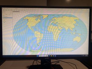
In Chapter 5, we began by learning about world map projections. We explored how geographic coordinate systems use latitude and longitude to identify locations on Earth’s surface, while projected coordinate systems apply mathematical transformations to project the curved surface of the Earth onto a flat surface. Next we gained experience using map projections commonly applied to the United States, learning that projections can preserve either shapes and angles or area, but not both at the same time. After that we learned how to set projected coordinate systems, and discovered that for medium and large size scale maps, it is best to use localized projected coordinate systems designed for a specific area to minimize distortion. We then worked with vector data formats, reviewing common file types used for vector spatial data as well as geodatabases, which we had previously done. Finally we learned how to download geospatial data for use in mapping and analysis.
Chapter 6:
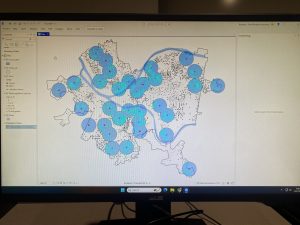
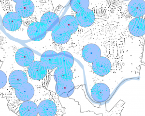
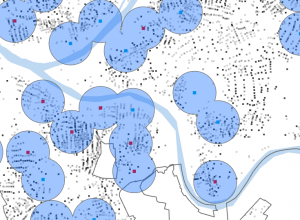
In chapter 6, we learned that geoprocessing is a framework and a collection of tools used to process geographic data. Geoprocessing tools are essential for building study areas within GIS and performing various analytical tasks. In this chapter, we practiced how to extract subsets of spatial features from a map using both attribute and spatial queries. We also learned how to aggregate polygons into larger polygons, append multiple layers to form a single unified layer, and use tools such as intersect, Union, and Tabulate Intersection to combine features and attribute tables for geoprocessing and spatial analysis.
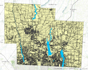
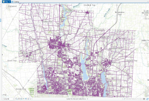
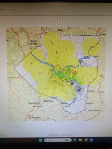
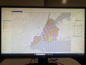
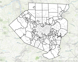
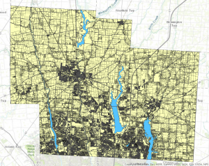
Delaware Data Inventory:
PLSS: All of the public land survey system polygons in both the US Military and the Virginia Military Survey Districts of Delaware County
Township: All 19 townships in Delaware County
Dedicated ROW: All right of way lines in Delaware County
Precincts: All voting precincts in Delaware County
Delaware County E911 Data: All addresses in Delaware County
Building Outline 2021: Building outlines for all structures in Delaware County in 2021
Original Townships: Original townships in Delaware County
Map Sheet: All map sheets in Delaware County
Farm Lot: All farm lots in the US Military and Virginia Military survey districts in Delaware county
Annexation: All Annexations and conforming boundaries, 1853 – now in Delaware County
Survey: Survey points that represent land surveys in Delaware County
Tax District: All tax districts in Delaware County
Hydrology: All major waterways in Delaware County
GPS: All GPS monuments from 1991 and 1997
Zip Code: All the zip codes in Delaware County
School District: All the school districts in Delaware County
Building Outline 2023: All the building outlines in Delaware County
Street Centerlines: The Center of Pavement of roads in Delaware County
Address Points: All the Addresses in Delaware County
Parcel: All of the cadastral parcel lines in Delaware County
Condo: All of the condos in Delaware County
Subdivision: All of the subdivisions and condos in Delaware County
Record Documents: All points of recorded documents in Delaware County