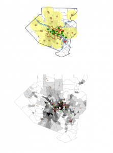
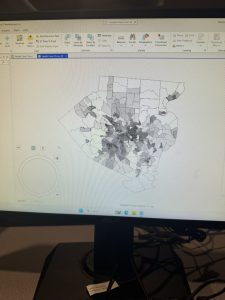
Chapter 1
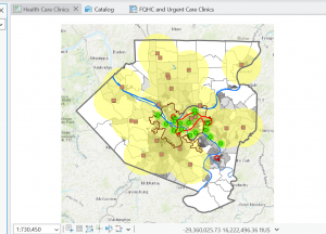
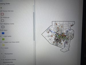
I found the straightforward walkthrough of the chapter extremely helpful in learning how to navigate the website. The chapter allowed me to navigate the different base layers and bookmarks in order to quickly access different features of the map that I needed. One key term that I found to be quite important was the word feature, which relates to a baseline quality to highlight different attributes of the map. Another would be Raster, which is an image made up of many small units called pixels, to make a much larger picture. A geodatabase is a folder that encompasses many other features and qualities of the map, which feels like an important term to know. Because of this chapter, I have become familiar with the top menu, which allows me to toggle between features in categories such as project, map, and more. It also taught me how to view the attribute table, which helps to put different boundaries into numerics, and you can even alter the formatting to show data more efficiently for your purposes. One question that had arisen for me when attempting to complete the tutorial was how to clear changes to a pre-existing column within the attribute table, as the option would become greyed out under certain circumstances. Overall, I had a positive experience with this chapter, and I appreciate how user-friendly it is.
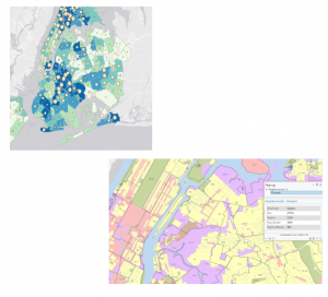
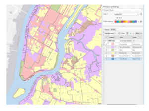
Chapter 2
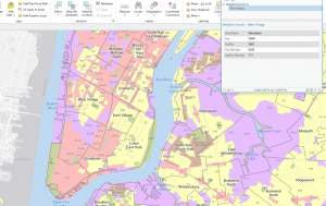
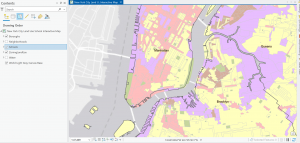
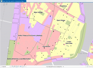
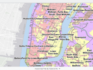
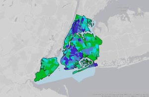
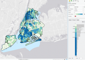
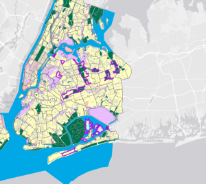
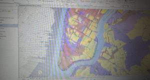
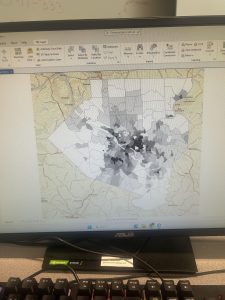
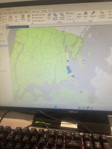
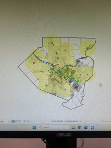
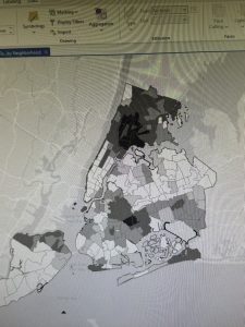
The second chapter has helped me to better understand how to utilize the symbolism and color preferences within ArcGIS. Not only that, but it has also explained the purpose of making the features a variety of colors and symbols in order to help the viewer better understand the contents of the map. The chapter also helped me to become familiar with the different labelling options and how utilizing a variety of fonts and colors for labels helps to make the map cleaner and more organized for the viewer. One question I have is what the cutoff is for too many different types of labels, in terms of formatting? More of would the viewer be more confused by too many different types of labels? I could definitely tell with this chapter that I was getting more comfortable with going through different tabs and accessing different features on my own, which I think is partly by design of the chapter, where, at least from what I noticed, they started lessen the amount they walked me through how to do certain basic actions that I had been taught in the chapters prior. Using a big city like New York helped me to better visualize the variety of labeling that can be used, and it was helpful to learn how to toggle visibility for labels depending on the current zoom. I had become very well acquainted with the symbology tab and the different terms of single symbol, unique symbol, graduated symbols, and dot density, which all feature the same data but with different visualizations.
Chapter 3
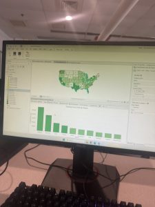
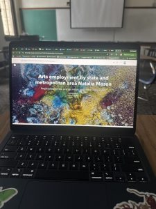
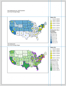
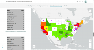
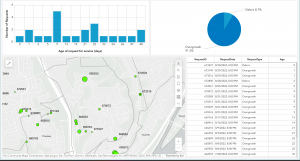
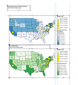
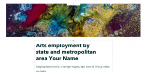
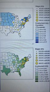
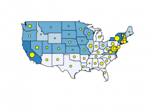
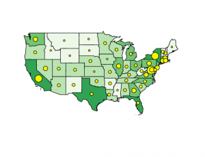
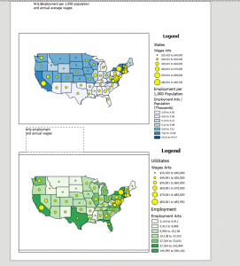
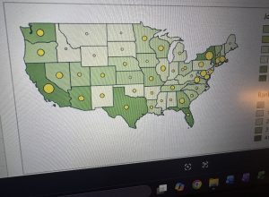
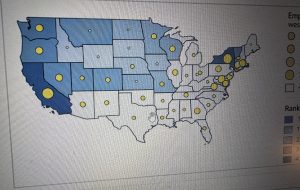
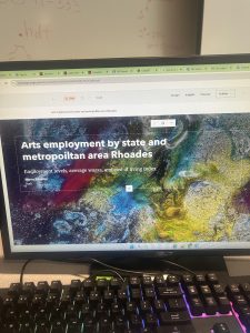
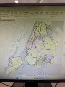
The third chapter delved deeper into the presentation aspect of the data, and how to do things such as format a layout to present information on a paper-like sample. I fear this was also one of the more difficult chapters thus far, as the tasks were less straightforward than those of mapping. I also found it interesting that it had also covered the aspect of creating storymaps to share with viewers. A story map is a type of online webpage that a user can post online to share map data and other topics of their choosing. One question I had when making the story map was where the catalog pane was, as within this chapter, I feel as though they were not as clear about that,t and I ended up having to look up how to find it. It also had me make a dashboard, which is another online visualization of map information, where it taught me how to create tables, pie charts, and bar charts. I found it quite interesting that I could edit so much of the map on the published online version, especially since it comes from such a large platform that a laptop typically can’t handle. The tutorial itself was mainly centered around Arts employment and cost of living wages throughout the U.S, and the clear way the data was presented made it intriguing to learn about.