Author: ajbenes

Chapter 9: 

• 9.1– Straightforward. I understood the applications. 
• 9.2– Pretty easy and straightforward, similar to the 9.1 application. 
• 9.3– In this tutorial I was having trouble changing the color of the polygons to the chips colors. I ended up changing them to a blue variation but didn’t understand where to find the needed color scheme. Once I got the calculate field in the polygon table I kept getting an error message and I don’t know what was going wrong. I couldn’t figure out how to continue once I got the error message. 
• 9.4– Easy tutorial. I understood the steps and application. 
• 9.5– I understood the contents of this tutorial. 

Chapter 10: 

• 10.1– Straightforward and easy to understand. 
• 10.2– When I put the symbology information in my map it had different colors than the book stated. This tutorial wasn’t too bad once I found where certain tools and applications were. 
• 10.3– Straightforward until. I got confused once I had to put in the expressions for the raster calculator. Therefore, I had to stop because I got confused and couldn’t figure out how to continue.
• 

Chapter 11: 

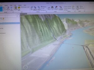
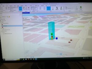
• 11.1– This tutorial was really cool to see the 3D dimensions and how to move the map in different ways. 
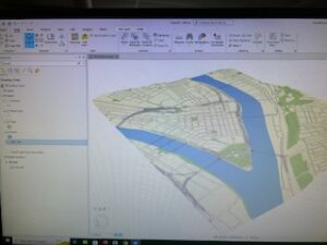
• 11.2– This was straightforward and I understood the process. It was interesting to see different layer colors. 
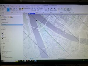
• 11.3– The create features tool wasn’t working and I wasn’t sure what was happening. Because of this I wasn’t able to fully complete the section. 
• 11.4–  Towards the end I couldn’t find the bridges in the created features. I was able to finish the tutorial but by the end portion my line of sight wouldn’t become 3D and I couldn’t figure out how to change that. 
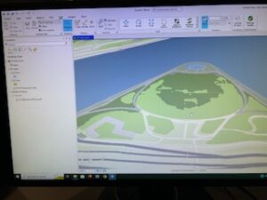
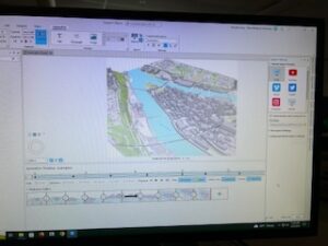
• 11.5– This tutorial went smoothly and was really cool to see the scaling aspect. 
• 11.6– This tutorial was going smoothly until I got the symbology pane. I was struggling to find this information. I was able to complete the rest of the tutorial. 
• 11.7– This was easy to understand and  really cool to see the animations. 

Delaware Data

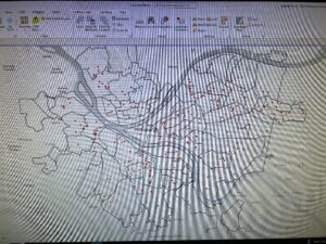
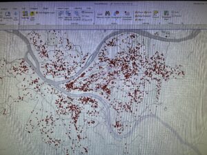
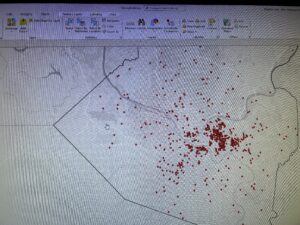
• Survey– This is a shape file that combines data from the recorder’s office and the map department. It was stated that the points on the map illustrate the survey plats.
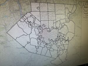
• MSAG– This data is known as the master street address guide. This data illustrates the 28 different political jurisdictions. This is used to find and analyze boundaries. 
• Parcel– This is data for the cadastral parcel lines in Delaware. These are represented by polygons. 
• Precinct– This data illustrates the voting precincts that are compiled by the county auditor’s office. Data is updated as needed. 
• Condo– This data shows all the condominiums in Delaware that are illustrated by polygons.
• Address Point– This data has all the certified addresses in Delaware. This data helps with emergency response, accident reporting and more. 
• Annexation– This is the annexation and conforming boundaries. This data goes back from 1853. 
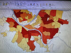
• Tax District– This data shows all the tax districts that are determined by the Auditor’s Real Estate Office. Data is updated on a need basis and published monthly.  
• GPS– This file has data from 1991-1997 for the GPS monuments. 
• School District– This data shows the school districts in Delaware. The data comes from the Delaware County Auditor parcel records.
• Zip Code– This shape file has all the zip codes in Delaware County. This shape file is published monthly to provide up to date information. 
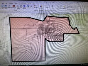
• Municipality– This is all of the municipalities in Delaware County. 
• Subdivision– This data contains subdivisions and condos that are in Delaware County. Data is published monthly and updated daily. 
• Building Outline 2021– This data has all of the building structures and was updated in 2021 and again in April 2023. 
• Delaware County E911 Data– This data is to help with the emergency response and accident reporting for Delaware County. This data shows the coordinates in relations to 911 agencies. 
• Township– This data is the 19 different townships that are in Delaware which are updated on a need-basis. 
• Recorded Document– This data is compiled of various information from surveys to boundaries and housing classification. This data is published monthly with weekly changes.
• Farm Lots– This shows all the farm lots for the US Military and the Virginia Military Survey Districts. 
• PLSS– This is the Public Land Survey System which shows the US Military and Virginia Military Survey Districts and certain boundaries. 
• Dedicated ROW– This data has the right of way information within Delaware County.
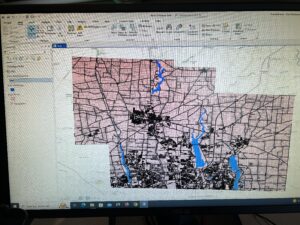
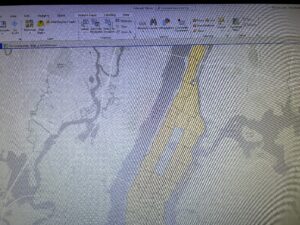
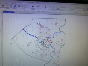
• Hydrology– This data shows the major waterways in Delaware County.
• 

Chapter 4: 

• 4.1– This was pretty straightforward and easy to understand. I learned how to create a new project and add necessary data. 
• 4.2– This started off strong but then I couldn’t find how to turn off base maps. I struggled to find the information in the tracts portion of this section. Therefore I just continued on to the next portion. I didn’t understand this tutorial, I think I might have messed something up or didn’t understand the wordings. 
• 4.3– This was a good section and it went smoothly. I felt that I was able to get a grasp of the concepts and what was happening. 
• 4.4– Short and easy. I was able to input the correct attributes and get the correct table. 
• 4.5– Easy to understand and straightforward. My map looked like it was supposed to and I feel confident in my ability to use this type of information. 
• 4.6– This section was easy to understand and wasn’t too difficult. 

Chapter 5: 

• 5.1– This was really cool to see the change from a flat map to a curved map of the world. 
• 5.2– I understood this section. I don’t know if this was just the program but when I would zoom in some of the states would disappear then reappear.
• 5.3– the beginning was easy. However once I got to the California UTM I couldn’t see anything on my screen. 
• 5.4– When I was working on the KML Data I got a notification at    the Geoprocessing layering failed. Not sure what went wrong. 
• 5.5– I struggled with the excel sheet. I couldn’t find the columns that were to be kept. For instance in Column JK it was (Estimate!!Female!!Workers 16 years and over!!..) whereas in the book it stated that Column JK Was (Male!!Estimate!!MEANS OF TRANSPORTATION TO WORK!!Bicycle). I couldn’t Finish this tutorial because I couldn’t get the data correct from the excel sheet resulting in me not being able to download and upload the file to ArcGIS Pro. 
• 5.6–  Straightforward and I understood the process of downloading shape files and inputting them into ArcGIS.

Chapter 6: 

• 6.1– I couldn’t do the pairing dissolve portion with the fire battalion. I am not sure why but It wasn’t running. I understood the process though. 
• 6.2– This wasn’t too difficult, however I did get stuck on the last portion. It wanted to pairwise cut but the correct file wasn’t on the dropdown menu therefore this process couldn’t be completed.
• 6.3– The process I am understanding but when I tried to merge the information for the waterparks, the system wouldn’t run the merge. I am not sure what I did wrong but I followed the previous directions. 
• 6.4– This section wasn’t too bad. I understood the concepts and found this easy to add the information into the attribute table. 
• 6.5–  This section was straightforward and I understood what I was working on.  
• 6.6–  I liked this section and it was going smoothly until the very end where I couldn’t merge the Brooklyn information together properly. 
• 6.7– Straightforward tutorial. I messed up with the running of the tool at the end but I figured out that I needed to select the file from the folder not just the dropdown menu.

Chapter 7: 

• 7.1– This one was easy and straightforward. I understood what was going on. 
• 7.2– This tutorial was going smoothly until I got to the part with the configure toolbar. I looked for it and couldn’t find it therefore I skipped that portion. After that the rest of the tutorial wasn’t too bad. 
• 7.3– Quick and easy. However when it got to your turn section I couldn’t figure out how to save the file into the folder. 
• 7.4– Pretty straightforward. However at the very end I couldn’t transform the building to the smaller version. The transform button didn’t show up. 

Chapter 8: 

• 8.1– I ran into an issue with the properties of the PARegion ZIP. However, after I smoothly got through the majority until getting to the rematching the addresses. I couldn’t figure out how to complete that because when I went through the steps it would just open the attribute table. Once I skipped over that step the rest of the tutorial went smoothly. 
• 8.2– This was straightforward and I understood the concepts.

Chapter 1: 

• 1.1 — Easy to follow once the website was up and running. I am not too technological but found that this wasn’t too difficult to understand with some help from peers.
• 1.2– The attributes were hard for me to understand at first but once I got a handle it was simpler. I really liked being able to see the variations that can happen in GIS
• 1.3– This was really cool to see the data and numerical values that the data has. I really liked being able to see the data and pinpoint where the information came from.
• 1.4– Couldn’t see the 3D map version and don’t know why. Might be that it needs to be updated. I am unsure of how to do that.

Chapter 2: 

• 2.1– I really liked going through the changing of the colors. I did end up with a slightly different looking map than the book has. I am not sure what I did wrong because I went through the same steps.
• 2.2– I really like how we are working with the labeling part because in the previous section I still wasn’t sure if I was doing it right. Therefore this made me feel more confident in my abilities.
• 2.3– Changing the symbols and colors wasn’t as difficult as I thought it would be. I am really beginning to understand the various methods to all the programing.
• 2.4– I began to struggle on page 45. And couldn’t move the tabs in the contents area. I didn’t know how to complete the rest of the exercise for this tutorial.
• 2.5– This one was short but I got stuck and couldn’t find the template symbol to change the squares to circles. Therefore I did it manually but then they disappeared from the map and I couldn’t get them the same color.
• 2.6– This was really cool to see the importing of data and to see various ways of navigating through the map.
• 2.7– I really liked changing the symbols and the corresponding titles. I feel like I am starting to grasp the program.
• 2.8– This was really cool to see the zooming in and out and how that can change what you can and cannot see.

Chapter 3: 

• 3.1– I struggled with this section. I couldn’t find the resizing and placing of the maps. I was able to create it but couldn’t find the areas for elements and properties. I couldn’t figure out how to move the map once I placed the ruler guides. I struggled with this tutorial and couldn’t fully complete it.
• 3.2– This was really cool to see the map on my computer and how it was able to be transferred onto the web version. I however couldn’t get the styles portion completed. It wouldn’t show up for me. I had a hard time working from the web version. I couldn’t find what I needed. 
• 3.3– It was cool to see more of the arcgis web version. I believe I did the posting and creation of the app correctly.
• 3.4– This was pretty straightforward. I did struggle with the pop-ups and therefore they don’t show up on the online version. Once it hit the adding of elements I lost some of the data and didn’t know how to continue.

Chapter 4: 

The beginning of chapter four talks about map density and how map densities are specifically used for finding patterns within the mapping; it also goes into depth about deciding what to map based on the data that you have. There are two ways of mapping density which are by a defined area, and by density surface. The chapter then goes into more depth about mapping density for defined areas which requires calculating a density value for these to find areas. The equation used for this is: population density = total population /(area/2787840). Further into the density for defined areas it talks about the dot density map And continues about the individual features that map density has for those to find areas. Next to the chapter talks about creating a density surface it goes into explaining the idea behind what the GIS does with the surface. In this portion there are a lot of calculations that need to be done such as cell size. For these calculations there are three different steps that need to be calculated in order to get that information. The next part of the chapter goes into displaying a density surface which pinpoints colors used for the maps. It suggests that because of the surface layering that there should be graduated colors to show the variation in the units that you are describing. it also goes into the ideas of Contours which are connection points of equal density that show the rate of change across surfaces. Lastly this part of the chapter talks about looking at the results and how you can understand and analyze the data that is being presented.

I really thought this chapter was very thorough. I am interested to see how we apply the calculations in this class because at first glance these calculations seemed a bit difficult to understand without knowing or seeing multiple examples of how those calculations are supposed to be used. 

Chapter 5: 

Chapter five starts off with why map what’s inside, it goes to the idea of being particular about what you’re deciding to bring to the data set. It talks about crimes that you can see in a certain area as well as toxic plumes. Understanding why someone would want to have this data set for future reference. Next it goes further into defining your analysis so going more into depth about what you can see and pull out from the data set especially if you’re looking at different areas in the book there’s single areas as well as multiple areas that are being discussed. therefore depending on what area you’re looking at it can determine what patterns or information you need to pull from it. After looking at the single and multiple areas it goes into the idea about are the features inside discrete or continuous. This just goes into the further investigation of the area to see if there is a big impact or less impact to the surrounding area. Following that explanation it goes into what information you will actually need to pull out from the data set starting off with the idea about needing a list count or summary. then going into more of the Strategic analysis of do you need to see these features that are completely or partially inside the area. This goes into the idea of the borders around that area and if something’s on that borderline do you count it or do you not count it. It was really interesting to see the comparing methods on page 147. This was really helpful in kind of the breakdown of what can be pulled from these maps and how they can aid in data analysis. The rest of this chapter just goes more in-depth about what can be found inside certain areas and features based on the data set and what information can be pulled based on the information that is present.  

Chapter 6: 

Chapter six starts off with talking about why map what’s nearby. meaning why expand the area that you’re looking at but then only focus on the smaller aspect. For instance if you are looking at an analyzing a small  neighborhood but you also have the outside roadways to see the traveling range of certain areas. then the book goes into how you’re measuring these areas and what measurements you should be using. They’re also different distances or cost ranges that you might need; these are inclusive rings and distinct bands. both of these pinpoint areas that you want your perspective audience to look at to grasp the data set that you are pulling from. In this chapter there was also discussion about creating a buffer within your map to make it more clear about where the information is coming from. There was also discussion about layering of information colors and more. especially when it came to creating distance ranges in various color layers. 

It was interesting to see on page 217 how you can have a bigger map but then designate two different areas of that map to have data point sets therefore you can kind of do a comparison about seeing certain data. On page 229 it was interesting to learn about the calculating cost over a geographic surface. I didn’t really know what this was and so it is interesting to learn that this is as stated from the book “Calculating cost distance over surface lets you find out what’s nearby when traveling overland.” I thought this chapter was really informative and gave really clear information about GIS mapping and the various maps that you can create and what data you can pull from those maps.

Chapter 1: 

Chapter one was the backbone of what GIS is and certain criteria that is needed for the application and data collection. GIS is used to see geographical patterns within data and relationships. Through GIS you can compile various datasets to create the results that are catered to your question you’re proposing. There are different layers to GIS that will create your data set such as features that will represent your data. These features are: discrete, continuous phenomena, and summarized by area. These features will create different maps based on the question you’re proposing and working with. GIS is about layering maps and information to create an end result. This means that on top of the features there are two different ways to represent the information which is vector and raster. On top of this information there are different ways of presenting the data points such as with percentages, numerical, pinpoints and more. A point was made in the book that it’s important to make sure the projections and coordinate systems are the same to ensure the data is presented correctly. All in all, GIS has many different factors that can be collected and compiled which makes each map and creation be different from one another even if they are focused on the same question. 

This was a really important chapter and with all the definitions and examples I am understanding more thoroughly what GIS is and how it can be used. The use of visual examples really helped me understand the content a bit better and I feel more prepared to work with GIS with this new information.  Some of the parts were confusing for me like the understanding of the difference between vector and raster. To me I just see that Raster is less clear and Vector has more definitive boundaries but I am not sure if there is more to the difference and use of them. 

Chapter 2: 

Chapter two was talking more about the in-depth understanding of the maps in GIS. There was information about putting your data into GIS and if a certain location isn’t already in the GIS platform, you do have to input it yourself manually. This means that you have to know the location information such as the street address or geographic coordinates. In this chapter there were descriptions about how you should designate your values, how they should be set up, the variations that come with that as well as the limitations. One of the limitations that was described was that a single map should not have more than seven categories. This resulted in being able to combine things that might be harder to put together which can change the outcome of the perception on the dataset. This limits the dataset because some areas shouldn’t be grouped together therefore it caused a disturbance in the creation of the dataset. Through this chapter it also talked about map skills which can really determine what catches the audience’s eyes such as having a zoomed in image of a map or a further away picture. In regards to the limitations of having only seven categories it was also talked about that sometimes having fewer categories can make the understanding easier but also have a more broader result. The final part of the chapter talked about analyzing Geographic patterns, which was really interesting to read about and seeing the variations that Maps can present and what data can be pulled from the data set. 

This chapter was mainly focused on zeroing in on mapping and points in which there were limitations benefits to certain areas as well as the orientation that map should have. I thought this was a really good continuation of the first chapter which really helped me understand the ideas behind GIS and what can be achieved from GIS analysis. 

Chapter 3: 

Chapter three elaborates on the ideas that were talked about in chapter two and dives into the comparison between most and least data sets. As well as focusing on why maps are important and what you can get out of that by summarizing certain data points. Another point that was talked about in chapter three was the idea of exploring the data or presenting a map. Which goes into why you’re creating this therefore understanding whether you need to accommodate it for other audiences or just tailor it to yourself. This chapter touches on just like chapter two did about the counts and amounts, ratios, and ranks, which are all quantities that can be utilized to illustrate information. Further in the chapter there was discussion about dealing with outliers, which is understanding the data set and getting to the most clear and concise map that you can have. It is possible that data sets will have outliers that will result in skewed data therefore they need to be analyzed and adapted to. The part about using charts was really surprising to see the visuals on page 90-91. The data sets were pinpointed as bar charts or pie charts. I had never seen anything like this before so that was something that caught my eye and I thought it was really interesting to see that you can make that type of dataset. This chapter also ended with the ideas of looking at patterns throughout GIS mapping which is really important.

I really thought this chapter connected very well with chapter two  and elaborated more on the points that were discussed in chapter two. It was also really  interesting to see the further understanding of GIS and how there are so many avenues that GIS can be used for in many different areas.

• I am Annabel Benes, a senior here at OWU, studying Environmental Studies and Business. I was born and raised in Denver, Colorado, I love to ski, hike and go on walks with my family and my dog Boscoe!
• 

• I took this course because I didn’t really use what GIS was and wanted to know more about what GIS is and how people use it around the world. This article was a very good background to the idea of what GIS is and what it can be used for around the world. It was interesting to see the benefits and consequences of GIS especially when it comes to different generational approaches for technology and learning. I didn’t know that GIS has been around since 1960, which seems like it was very before other high end technology. Figure 1, was similar to me because in the fall semester I took soil morphology where we saw a map where we wore specific glasses to have a 3D vision. The maps from Soil Morphology were layered but you could only see the various layers with the specific glasses on which was really cool to see. The layers of figure 1, seemed very similar to the idea of this map in that class. I could visually see all the layers in a different form but still could understand the layout of the picture and what it represented. From this article it seems like GIS is just a big bundle and online version of data points and information from around the world. I found it interesting that you can combine different variables to get the data that you are trying to examine. Like with figure 1.4, seeing the correlation between pumps and cholera cases. I enjoyed reading about this introduction to GIS and I am excited to gain more information and understanding of GIS. I do have questions after reading this: How often is GIS information updated, for instance the layout of the ground, buildings and more? I also would like to know what tools can be used to create this data and if there are faster tools that are being created? 

• One source that I found was wolf tracking and the role of surveillance in the recovery of an endangered species, from ArcGIS. This was really interesting to read about and see the maps for tracking. The article specifically focused on Gray Wolves and their recovery and survival throughout the years after being put on the endangered species list. This article focused on Washington area and attached is the map that they collected from the tracking:
• 
• From another article it stated that in Washington State, “ Washington is home to about 33 packs. Nineteen of these packs have successfully bred. The Department of Fish and Wildlife has enforced laws to manage conflict with people over livestock predation by wolves. Because of these efforts, there are about 200 wolves in Washington.” https://worldpopulationreview.com/state-rankings/wolf-population-by-state 
• Another application that I found interesting was using GIS to study rivers. I think it’s really interesting to see where rivers were and where they are now and what changed their path. This was a short article that illustrated the basics of the study. https://serc.carleton.edu/eyesinthesky2/week6/study_rivers_gis.html 
• From this initial search I went deeper into finding maps of rivers in Ohio. From ArcGIS I was able to see rivers, canals and more in Ohio which was really interesting. Attached below is a snippet of the map that I looked at:  
•