Andisman, Week 5

Chapter 4: File Geodatabases

4.1 + 4.2

• File geodatabase: Esri’s simplified database for storing geospatial data, including features, classes, and raster datasets for single users for small groups
• In ArcGIS, data management and processing in a file geodatabase is done through the Catalog pane -> tools -> user interface
• They have no practical limits for numbers and sizes of feature classes or raster datasets stored in them, and are optimized for data processing and storage in Arc. They also allow data tables to be related and joined 
• Note: Attribute, Field, Variable, and Column are interchangeable names for the columns of data tables
• Note: Record, Row, and Observation are interchangeable names for the rows in a data table
• Shapefile: A spatial data format for a single point, line or polygon layer. 
• Connect a data folder through the catalog pane -> folders -> right click -> add folder connection
• Shapefiles need to be converted to a feature class and stored in a geodatabase because it doesn’t support advanced capabilities. Do so with the export features tool in the geoprocessing group in the analysis tab
• Deleting tables/feature classes from a file geodatabase is permanent, but removing a layer from the Contents pane removes it only from the map and leaves the feature class in a file geodatabase
• Fields in a data table in gray font are essential and cannot be modified
• Joining tables requires each table to have an attribute with matching values stored with the same data type

4.2 Note: A bug in 4.2 with ‘Tracts’ I think? Something weird going on here, got through as far as I could, but data was not showing up and it would not let me get past running the calculation of the sum of fields for PopYouth.

4.3

• Attribute queries are based on SQL
• A simple criterion has the following form: 

attribute  name <logical operator> attribute value

• The attribute name can be any column heading or field name in the attribute table, and several logical operators are “ =, >, <, =>, =<”. The attribute table specifies what you’re looking for. For example: the following simple criterion selects all cries that are robberies where robbery is a value of the crime attribute:    Crime = ‘Robbery’ 
• Numeric fields do not need quotation marks like text does
• OR and AND can also be used to select and specify criteria
• The use of parentheses, like in algebraic expressions, is essential because logical expressions are run one pair at a time for simple expressions, generally working from right to left, but with certain logical operators going first, such as AND being run before OR. This can result in incorrect information unless you use parentheses to control the run order
• Crime analysis use three kinds of attribute queries: ‘What and when”, specific when such as time of day, and specific who or what or how 
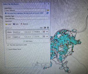
• Queries for event locations, such as crimes, almost always use date-range criteria
• The ‘qry’ prefix is the standard prefix for database inquiries

4.4

• Spatial join tool was easy 🙂

4.5

• The centroid pf a polygon is the arithmetic mean of all points within the polygon. If you want all center points to lie within their polygons, the remedy in ArcGIS is to use central points instead of centroids

4.6

• Sometimes a data table has a field name that uses a code that, by itself, isn’t easily understood. Therefore, you need a code table with all the codes in one field, along with their descriptions in the second field. This join is called a one-to-many
• Use the Create Table tool
• 

Chapter 5 Spatial Data

5.1 

• Geographic coordinate systems use latitude and longitude coordinates gor locations on the surface of the earth, whereas projected coordinate systems use a mathematical transformation from an ellipsoid or a sphere to a flat surface and a two dimensional coordinate
• Geographic coordinates are angles calculated from the intersection of the prime meridian and the equator. 
• Longitude measures east – west and ranges from 0 to 180 degrees, latitude measures north and south and ranges from 0 to 90 degrees
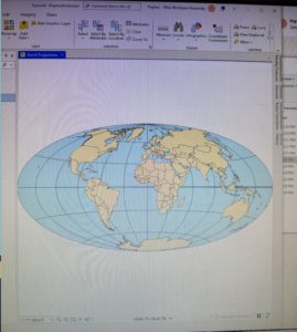
• The network of lines on the map os called a graticule and has 30 degree intervals east – west and north – south
• The Robinson World projection is the most accurate at the mod latitudes in the N and S hemispheres where most people live, and minimizes distortions 

5.2

• When working with projections, you can either get accurate shapes/angles or accurate areas, but not both at the same time
• As a rule, use projections that give an accurate area (even if it causes some distortion in shape or direction), such as the Albers Equal Area or the Cylindrical Equal Area projection. Albers is the standard for the US Geological Survey and the US Census Bureau

5.3

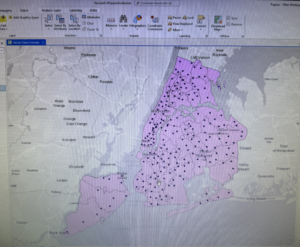
• For medium and large scale maps, use localized projection coordinate systems tuned for the study data, that have little/minimal distortion
• This tutorial set the projected coordinate system (state plane) for a local map by adding the first layer to the map and specified the display units
• The first step to using the State Plane coordinate system is to look up the correct zone for your area and the specific projected coordinate system tailored to your study area
• You can set the default coordinate system using the Choose Spatial Reference option, regardless of what layers you add to it

5.4

• A shapefile consists of at least three files with the following extensions: .shp, .dbf, or .shx
• Shp file stores the geometry of features, dbf file stores the attribute table, and shx file stores an inde of the spatial geometry
• X = longitude; Y = latitude
• KML file is the file format used to display geographic data in many mapping applications, is an international standard, and maintained by the Open Geospatial Consortium
• KML files can be converted into a feature class by inputting the KML in the KML to Layer Tool, outputting to the data file, and then naming the  new data file.

5.5

• Discrepancy with the data we have to download from the internet compared to what is written in the book for Tutorial 5-5. Column JK written in the book for the “male transport to work via bicycles” is actually column EG or code S0801_C02_011E on the spreadsheet. Column SE in the book for “female transport to work via bicycles” is actually Column IQ on the spreadsheet.
• Lots of free data is available to download from the US Census Bureau website
• Using Topographically Integrated Geographic Encoding and Referencing shapefile (TIGER)

5.6

• You can download data from many government websites such as the USGS National Map Viewer  or Data.gov, or USDA, DOC, NOAA, US Census Bureau, DOI, EPA, NASA, ArcGIS Living Atlas of the World
• This chapter involved searching for and adding a land use raster layer from ArcGIS Atlas
• In ArcGISPro, you can add data from the atlas using Catalog Pane -> Portal -> Living Atlas (or the Add Data button)
• Rasters are large files
• If you want to extract a subset of data, use the Extract by Mask tool
• 

Chapter 6 Geoprocessing

6.1

• Geoprocessing is a framework and set of tools for processing geographic data. Generally, it must be used to build study areas in GIS and perform tasks. 
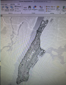
• This section focused on dissolving features, which retains the outer boundary lines bt removes interior lines from the block groups
• The Pairwise Dissolve tool can aggregate block group attributes using statistics such as sum, mean, and count. The PwD Tool needs data as the Dissolve Field. For example ‘Name’

6.2

• This section worked through extracting and clipping features for a study region when there were more features than needed by first creating a single polygon, using the new polygon and select by location to create features of block groups in the study area only, and then use the Clip Tool

6.3

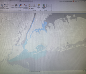
• This section merged several adjacent water features to build oe water feature as a single layer by using the Merge Geoprocessing Tool

6.4

• The Append Tool adds features to an existing feature class, considering that both have the same attributes, or the same schema
• The schema is the table (field) structure. This allows you to choose the option for matching the input table’s schema to the target table’s schema

6.5

• The Pairwise Intersect Tool creates a feature class combining all the features and attributes of two input (and overlaying) feature classes, like fire companies and streets
• The Intersect Tool excluses any parts of two or more input layers that don’t overlay each other
• Studying the attribute tables of each feature class familiarizes you with the attributes before you intersect features
• After intersecting features, you can go through the attribute table to create a summary with the Summary Statistics Tool

6.6

• The Union Tool overlays the geometry and attributes of two input polygon layers to generate a new output polygon layer. This can be useful for things like urban planning, allowing you to calculate things like land use type
• The Calculate Geometry Attributes Tool can be used for calculating value such as acreage

6.7

• The Tabulate Intersection Tool makes estimations by making apportionments proportional to the areas of split parts of polygons, such as block groups, and assumes that the populations of interest are uniformly distributed by an area within polygons
• 

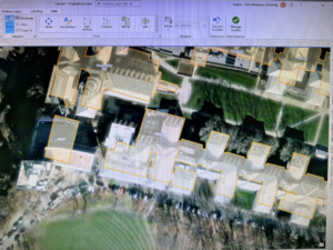
Chapter 7: Digitizing

7.1

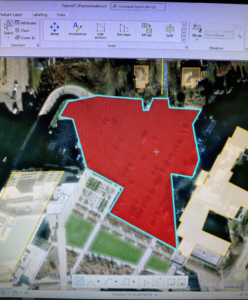
• This section introduced the editing process for existing facets of a GIS map, specifically, the editing of polygon features, by splitting polygons, through the addition of vertex points, and revising them to match existing features such as a building on the World Imagery Basemap. 
• To move a polygon, use Select and then under the tools section in the Edits tab, choose move to adjust its position
• To rotate a polygon, select it, click ‘Move’, and then in the Modify Features tab, choose Rotate
• Vertex points can be added to reflect a building’s true shape. Select by the same steps, but under tools, choose Edit Verticles
• Polygons can also be split using the “split” tool

7.2

• Point and line feature classes can be created with similar steps
• Polygon features can be created and deleted
• Feature classes can be created directly from the Catalog pane and attributes can be added, but the Create Feature Class Tool could instead be used with attributes later added in the attribute table
• Select and use the “Delete” button under the Edits tab to delete polygons
• The Trace Tool creates a polygon using parameters like streets as guidelines

7.3

• A useful tool to improve the aesthetic or cartography quality of polygons is the Smooth polygon Tool. 
• Smoothing Tolerance: A shorter length will result in more detail, but will take longer to process

7.4

• Computer Aided Design (CAD) are commonly used but not geographically referenced to a coordinate system
• Transforming features in GIS makes aligning CAD drawing to GIS maps easy, regardless of the coordinates and units
• CAD drawings contain color coded layers. You cannot edit CAD drawings directly, so you have to export them as a feature class by right clicking the polygon in Contents -> Data -> Export Features. The saved polygon will be automatically added to Contents, and the old CAD can be removed
• The result of exporting a CAD drawing are that the properties of the drawing are added as fields in the attribute table. To alter this, use the Apply Symbology From Layer Tool
• 

Chapter 8: Geocoding

8.1

• Geocoding is a GIS process that matches location fields in tabular data to corresponding fields in existing feature classes. Examples include street addresses + zip codes, or transaction data collected by organizations. 
• The software uses Algorithms to identify possible incorrect entries for things like misspelled street addresses and attempts to problem solve inconsistencies.
• The following components are used: Source table, reference data, geocoding tool, locator
• A geocaching locator is a set of files that stores parameters and other data for the geocoding process. Use the Create Locator Tool. High parameter values allow fewer match errors, while low parameter values allow more match errors. 
• Geocode Address Tool can be used to use geocode data by zip code
•