Preface +Ch.1: Before reading the book I was very nervous to start using ArcGIS Pro because I am not very good with technology. However, after reading the preface I felt reassured primarily because the book was set up in a step-by-step format. Therefore, I was very relieved when I noticed that chapter one was specific with its instructions and how to use the app, especially with finding the tabs, panes and other items. Despite these specific instructions I still struggled with finding these buttons but that could be due to my eyesight. That made the tutorial longer, but eventually, I believe I was able to manage most of the GIS settings and projects. Nonetheless, I would like to start working ahead with the other tutorials in order to avoid feeling overwhelmed.
In this chapter, I learned that the file geodatabase is a folder that stores features and raster’s etc., meanwhile a project is a file that contains maps and related files. I also learned that the GIS software is able to detect certain features depending on the order they are displayed. Thus, the feature at the bottom of the pane is displayed first and then the layers above it are displayed afterwards. I learned that features that cover larger areas should be at the bottom of the list. I also believed that having buffers available was a good way of demonstrating the relationship between features, especially because they are transparent. Another interesting part of ArcGIS Pro was being able to see some features when you zoomed in on the map. This reminded me of Google Maps, where you can see individual street names or locations the closer you zoom in. Despite my technological struggles, I was happy to experience the basics of GIS and I hope to improve both my GIS and technological skills. I was able to improve on them throughout the other chapters, but I could always use more practice.
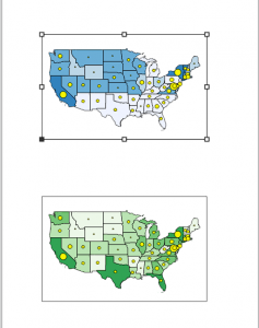
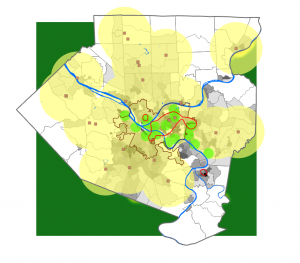
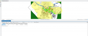
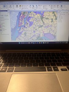
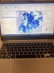
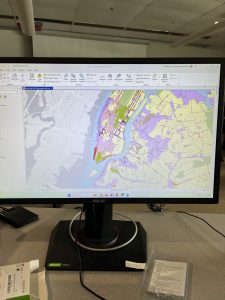
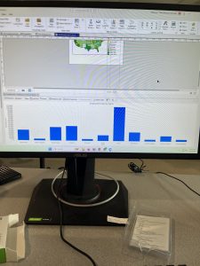
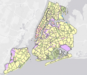
Ch.2: In chapter two I was able to learn how to add symbols and characterize my map. I learned that a thematic map can be used for solving a problem and consists of many layers. The importance of this map is to ensure that the features are identified as figures since it makes up the majority of the map. Otherwise, if a feature is not identified then the GIS will count it as ground. Part of the first tutorial was to display symbols for the New York map, which was fun because I really like colors. Although, for some reason the water on my GIS map was not turning blue, everything else was fine. In the third tutorial I also learned that a definition query is used to limit the features to a subset for a large collection. It is used to filter features of a layer instead of temporarily selecting features to work with. Throughout the chapter, I also noticed that some terms such as natural breaks, and quantile from the first book are mentioned. Furthermore, I also learned how to create a histogram which was interesting.
Even though this chapter was fun to explore especially with the colors, I still had technological difficulties. Throughout the chapter the instructions began to be less specific, especially when it came to the “Your Turn” exercises. I understand that these were meant to put into practice what we learned from the tutorial but since I don’t understand computer software and have bad vision, it was hard to complete it. Other times, the system would not allow me to fully complete my tasks so I had to skip some of the instructions. I still read over them to get an idea of how the features were supposed to work, so I would not fall behind.
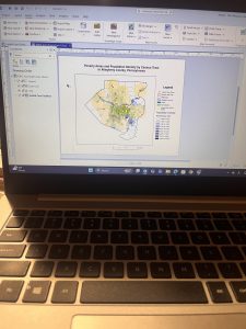
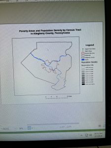
Ch.3: Throughout this chapter, I still struggled with the software at times but I still read through what I needed to do to make sure I understood what was going on. I also noticed that at this point the instructions were a lot less specific compared to the first chapter. Personally, I noticed that the wording for some of the instructions were complicated and it did not make much sense to me. Especially when it was referring to the sizes of rulers, guidelines or legends. Another confusing part of the tutorial was when the instructions mentioned zooming in on a specific area on the map. Sometimes I would forget to use the bookmark system to zoom in on a location, which led me to manually do it and I would get confused when comparing my map to the example map. I do not think it was entirely required, but it would have been useful to have the same map section as the reference.
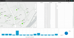
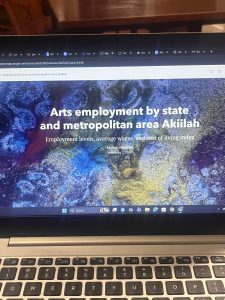
I also thought it was useful to learn how to create a story and post a map on the website. This is useful because it may be helpful to share information with others, especially when it comes to expanding research. I believe that being able to have this source is helpful for students overall,when it comes to sharing data, giving credits and asking for help during the research process. Towards the end of the chapter I was also able to learn how to create a bar graph using the map. At the end of all the chapters and tutorials I realized that there was a lot of statistics and graphing involved with GIS. As well as repetitive actions in order to change a certain symbol or feature. Nonetheless, I enjoyed the creativity allowed within the software and I hope I will continue to enhance my knowledge.