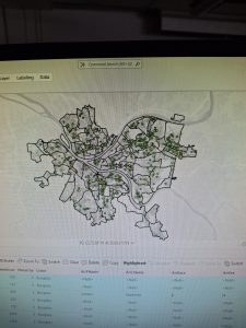
Agrawal Week 5

Week 5

Chapter 4

Chapter 4 helped me understand how much of GIS work happens through the data behind the map, not just the map itself. I worked more with attribute tables, fields, and joining data from different tables. I also learned how to calculate new fields and use the data to display specific information on the map. At first, keeping track of the different tables and fields was a little confusing, but once I could see the changes reflected on the map it made a lot more sense. I think working with attribute data like this will be useful because it lets you take a large dataset and actually pull useful information out of it.

Chapter 5

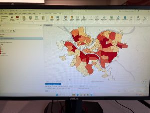
Chapter 5 focused more on spatial data and the different ways geographic information can be stored and brought into ArcGIS Pro. I worked with coordinate systems, projections, shapefiles, XY coordinates, and other data sources. One thing I noticed in this chapter was that there are a lot of small steps involved in getting outside data into the right format before you can actually use it. The Census data section especially showed how data from another source can be joined with geographic features and then represented visually on a map. Some of the steps were harder to follow because the book does not always match the current version of ArcGIS Pro exactly, but figuring out where the tools had moved also made me more comfortable navigating the software.

Chapter 6

Chapter 6 felt more focused on actually analyzing and combining the data that was prepared in the earlier chapters. I used more geoprocessing tools, including tools for selecting, merging, clipping, and intersecting features. I thought this chapter made the purpose of some of the previous work clearer because instead of just adding information to a map, I was using different layers together to answer more specific questions. The tabulate intersection work was also interesting because it showed how GIS can calculate information based on where different geographic areas overlap. There are still a lot of tools and options that I would probably need instructions to remember right now, but I am starting to understand what the different tools are actually doing instead of just following the steps.

Agrawal Week 4

Week 4

Chapter 1

Chapter 1 was mostly about getting familiar with ArcGIS Pro and learning how to navigate the different parts of the software. We worked with layers, attribute data, symbols, labels, and both 2D and 3D maps. The health care clinic example was interesting because we could look at the locations of clinics along with other information about the area instead of just seeing points on a map. I also liked the 3D population density map because the differences were easier to visually notice when they were represented by height. I did have some trouble finding certain tools because there are a lot of different tabs and options in ArcGIS Pro, but going through the tutorial helped me get more comfortable navigating it.

Question: When is a 3D map more useful than showing the same information on a regular 2D map?


Chapter 2

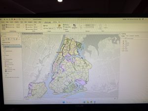
Chapter 2 focused more on how the information on a map is actually displayed. We worked with symbology, labels, choropleth maps, dot density, and visibility ranges. One thing I found interesting was how differently the same type of data can look depending on how it is symbolized or categorized. For the New York City land use map, the different colors made it easier to distinguish between types of land use such as commercial, manufacturing, parks, and residential areas. Having the borough and neighborhood boundaries along with the land use data also helped give the map more context. This chapter was a little more difficult for me because some of the options in ArcGIS were not always where I expected them to be, but I got more familiar with working with layers and their properties.

Question: How do you decide which type of symbology is best for a dataset without making the map too complicated?


Chapter 3: Maps for End Users

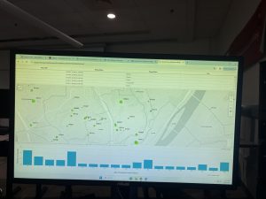
Chapter 3 was different from the first two because it focused more on how GIS information can be shared and presented to other people. We worked with layouts and also used ArcGIS Online tools such as StoryMaps and Dashboards. I liked seeing how the work done in ArcGIS Pro could be used in an online format instead of only staying inside the desktop application. The Ground Crew Dashboard was probably the most interesting part for me because it put several ways of looking at the data in one place. The dashboard included the locations of service requests on a map, information about individual requests in a table, and a chart showing the age of the requests. Seeing these together helped me understand how a dashboard can make geographic data easier to look at and understand without needing to work directly in ArcGIS Pro.

Question: When would a Dashboard be more useful than just sharing a regular map?

Boldman Week 5

Chapter 4

Chapter 4 taught me how to organize further and modify attribute data using a map. I can remove unnecessary fields and calculate new values, which can lead to joining tables and make data easier to analyze. This skill is important for future work with GIS because I can zoom in on data in large map work.

Chapter 5

Chapter 5 introduces different types of spatial data and how to convert them into different formats. Some of the files I worked with include shapefiles, XY coordinates and KML files, which allow for different sources to be combined and displayed accurately on a map.

Chapter 6

The lessons in Chapter 6 taught me how to combine, add, and analyze various geographic datasets. I learned to use new tools such as Merge, Dissolve, and Intersect. These tools will be beneficial in the future when I want to streamline the amount of data I am working with


Data Inventory

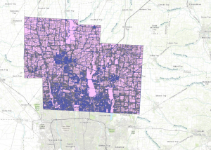
1.  Annexation:  Published monthly and consists of all of the annexations and boundaries from 1853 to now.

2. Street Centerline – A layer in the GIS map that shows the center of the roads in Delaware County.

3. Recorded Document – Points of data representing documents in Delaware County not included in subdivision plats that are active. Data is facilitated in a process of locating miscellaneous documents.

4. Survey – A shapefile including point coverage representing surveys of land in Delaware County.

5. GPS – Identification of points established between 1991 and 1997 and is published monthly.

6. Subdivision – Data consists of condos and subdivisions recorded in Delaware County Recorder’s Office. Data is updated daily and published monthly.

7. School District – Data holds all of the School Districts within Delaware County.

8. Tax District – This data set consists of all tax districts within Delaware County and is defined by Delaware County Auditor’s Real Estate Office.

9. Parcel – This dataset consists of polygons that represent all cadastral parcel lines within Delaware County, Ohio. The cadastral geometries are maintained by the Delaware County Auditor’s GIS Office.

10. Township – The dataset includes 19 different townships making up Delaware County and is updated on an as-needed basis.

Meyst Week Five

Chapter Four Notes:

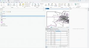
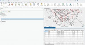
Chapter Four was a fairly difficult chapter to complete, introducing concepts from the previous three chapters along with a tutorial on how to create your own project. I found creating my own project to be fairly difficult to begin with, as the other tutorials are all provided for the reader. However, by Tutorial 4-2, I felt far more confident with creating my own basemap and project and importing the data provided. Unlike the Chapter Three tutorial, where the reader was generally provided with copy-and-paste data, in Chapter Four, there was far less guidance on a new subject. The rest of Chapter Four mainly dealt with becoming comfortable and familiar with ArcGIS as a software, especially in terms of familiarity. In Tutorial 3-3, oddly, when calculating specific burglaries by different filters, the burglaries were off in terms of count. The textbook lists the count of burglaries as 273, with 84 occurring on the weekend. However, my count ended up as 309, with 75 occurring on the weekends. This was after I double-checked my search query for the correct date and crime. Further, the query person attributes had inaccurate values displayed. Otherwise, Chapter Four relatively followed the textbook, and I had to make no major adjustments to the commands provided in order to complete the work in the textbook.


Key Commands and Concepts Taught In This Chapter:

  • Add join: Joins two datasets together, merging data tables to be able to complete or calculate fields in relation to both tables and data sets
  • Create table: Uses pre-existing map data and condenses it into an easily editable format for further data analysis and manipulation
  • Calculating the sums of fields: adding, subtracting, etc to different data sets in order to calculate a percentage or other form of data presentation. Relies on basic Python script
 

Chapter Five Notes:

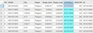
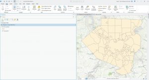
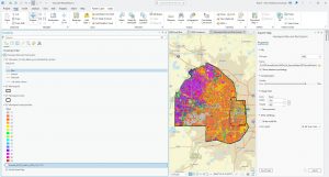
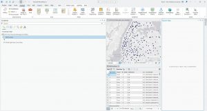
Chapter Five took me the longest amount of time and outside research due to inaccuracies in the textbook that make following the textbook directly impossible. Tutorial 5-1 through Tutorial 5-3 were fairly straightforward, and only took me about ten minutes each to complete. Much of the first half of Chapter 5’s tutorials are reviewing key concepts covered in previous chapters, and only take a few commands to complete. Additionally, this first part of the tutorial teaches incredibly vital map skills, which I went back to review multiple times in the following tutorials and also within completing the tutorials for Chapter 6. Tutorial 5-5 was very different from what I was used to in the preceding tutorials and chapters, as I have never worked with Microsoft Excel or other similar programs such as Google Sheets. Editing the data was fairly straightforward, and I found that highlighting the columns that I needed to avoid deleting in red text made it much easier to not lose the columns in the rest of the data set. Further on in this tutorial, I found that the command provided to join together the MinnesotaTracts and BikeWorkData tables were very incorrect. The GEOID and GEOIDNUM fields both registered as incorrect when placed in the Input and Join Table fields, and were instead placed in the order: MinnesotaTracts > GEOID > BikeWorkData > GEOIDNUM. As completing the Add Join function was vital to the rest of the tutorial, adjusting the command was necessary. In the next chapter, the tutorial erroneously lists the basemap used, which took some adjustment and guessing in order to accomplish.


Key Commands and Concepts Taught In This Chapter:

  • (For my own further review) The pathway to change the map projection for a basemap is: Contents > Properties > Coordinate System > Projected Coordinate System. This contains multiple world, US State, and country projections.
 

Chapter Six Notes:

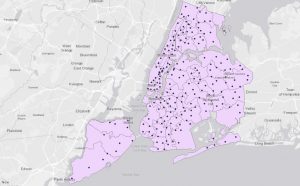
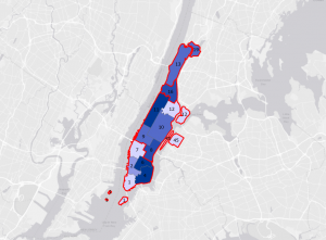
After many major adjustments to Chapter Five’s listed commands, I was relieved to find that Chapter Six had no major errors unlike the previous two chapters. Whether the outdated version or some other factor, the previous chapters very much tested my computer knowledge! Chapter 6, notably, uses far less descriptive wording than the introductory chapters, which was initially a bit of adjustment in remembering how to execute certain commands without express guidance from the textbook. For example, in the very first tutorial, the textbook asks the reader to label the New York fire stations by district. Initially, I forgot which commands were required in order to label a certain area, and I had to repeatedly undo actions I took until I was able to review and correctly label the map. Additionally, a previously introduced feature which I had some difficulty remembering how to execute was the Select tool. It took me multiple tries to realize selecting a certain feature was just clicking, not necessarily dragging the cursor over an area, which selected too many attributes. Then, while saving the selected section was not reviewed, I was able to parse out what function was required in order to save a selected area. Most of the tutorials in this chapter dealt with learning what to input for certain commands, especially key commands used frequently throughout the textbook.


Key Commands and Concepts Taught In This Chapter:

  • Merge tool: merges multiple datasets into one feature that is easier to edit and symbolize, for example, merging together all portions/neighborhoods of New York City to create a comprehensive map of all of New York City.
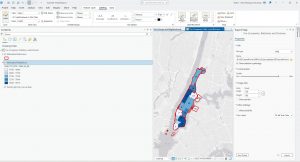
  • Tabulate Intersection: estimates the number of people within two boundaries, shown in the textbook as census boundaries and fire station districts.
 

McMahon week 5

Chapter 4:

From chapter 1 a lot of the key focuses were to create attribute tables and add data into the map. I was able to label the data and download it from other sources but it was difficult to find the folders in which they were in and import them. But I was able to get it after a while and edit the map.I was able to work with spacial databases and I thought that this skill was important.

Chapter 5:

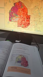
This chapter focused more on locations and longitudes and latitudes. It got easier as the chapter went on because I started to figure out where somethings were. But I did get lost in some areas because the chapter started to assume I remembered the steps, but I still need the step by step process. Some problems came up with the end of each chapter and I thought that the “Your turn” sections were confusing. I thought these maps were interesting thought because I could actually see a difference by the end of the section. The Microsoft section was also confusing but I thought it was good to get some experience in this area. This chapter used censuses.


Chapter 6:

This chapter was a lot easier than the chapter 5. I was able to make attribute tables and edit the input and outputs of the data. By the end of the chapter it was pretty easy to assume the same steps were going to be taken. I was able to use Pairwise tool and get familiar with it. Overall I think this chapter allowed me to get familiar with tool searching and making tables.

Robinson Week 5

Chapter 4:

This chapter covers spatial and regular databases. Using the .gdb extension, which is not a file extension but merely a folder. The first section starts us off by importing data into a project. Next using the capabilities of a database in the Catalog pane. This allows us to alter or copy geodatabases. The chapter mentions the importance of columns in data tables, where most attributes are handled. 4-2 discusses modifying attribute tables, using the calculate field tool (I found this part a bit confusing but later figured it out), and joining/exporting features. The same section also shows how to calculate fields and draw out/concatenate (basically combine; e.g., “Bob” + “Bob” = “BobBob”) string fields. The section after I thought was the most interesting, where we connect data from tables to feature classes. This is done with SQL queries regarding filtering, which contain 3 parts: the attribute name, a logical operator (<, >, etc.), and an attribute value. (Haven’t heard of SQL since my Intro to Database Fundamentals class a good minute ago.) There are 2 types of queries: simple and complex. Simple queries use 1 connector, while complex queries use 2 or more. Connected by the operators an and, or, an or. Queries can be used to filter out features based on certain characteristics like age, time, (in this chapter) type of crime, and location. Section 4-4 was a short section on how to aggregate data with spatial points. Later, the chapter showed us how to use central points for shapes. I thought of this as basically adding a dot, where the dots represent the number of burglaries by neighborhood. The last section of the chapter had us create a new table to help the user simplify data by reducing duplicates. Overall, I thought this chapter was pretty interesting to work with.

Chapter 5:

In the last chapter, we learned about filing geodatabases; in this current one, we learn more about spatial databases specifically. In the first section, we used coordinates and changed world map projections. I think I spent maybe 20-30 minutes looking at all the types of projections that the GDB file had to offer. The next section had us working within the subject, but within the U.S. Not only that, but the chapter also discusses how to set reference zones to help select projected coordinates. Based on what area the user wants to study. One of the most interesting things I learned from this chapter was how to add new layers on a coordinate system. Later, we changed the map coordinate system; this process was pretty easy. I originally thought it would be harder than that, or at least more complex. The following section has us working with vector data formats. This required importing a shapefile, adding x and y coordinate data, and finally converting a KML (Keyhole Markup Language) file into a feature class. 5-5 really gets into real-life data through the U.S. Census, requiring us to download specific data sets. I never even knew a website like that could exist. I also spent some time going through the website, checking the menus and data from other cities. After all this information was downloaded, it was entered into GIS. This section took the longest because I messed up a step along the way and had to repeat the process. When all the information is gathered, the collected data is joined and turned into a choropleth map. Learning how to download geospatial data was pretty straightforward, as was adding it to the current map. When this chapter was finished I explored some agency maps, this specific chapter piqued my curiosity.

Chapter 6:

In the previous chapter, we learned to search through geographic databases, either by collecting the information ourselves or through another source, like a government agency. The sixth chapter focuses heavily on geoprocessing and its use cases to build our areas of study. The first section of this chapter had us delete features to create new ones using the Pairwise Dissolve function. This totals the attributes using statistics like count, sum, and mean. Next, we clip (a geoprocessing tool) and extract those features for the purpose of studying them. By using Select By Attribute (this part was easy) and the Select function, a bit annoying to use because I couldn’t figure out how to use it correctly. After that, we combined water features using the merge function. This tool basically combines two or more feature classes into one. Then we used the Append tool to add data from one source to another dataset. (Haven’t heard this word since my Python Class maybe a year or two ago.) Next, we intersected those features to determine their specific zones. This part of the chapter uses the Pairwise Function once again but with a new tool called Intersect. This new tool removes any input layers that do not overlap. Then we use a tool called Union to overlay the attributes and space of specific layers to create a new one. Finally, the chapter closes out with us using the Tabulate Intersection. The results show us the calculations of how map layers overlap, which it outputs in the table. Overall, I thought this chapter was a bit complex, but I learned a lot from this part of the book. The complexity comes from performing a bunch of new tasks with newer functions. As well as learning what these new functions specifically do and their uses.

Bruner Week 5

Throughout this week’s tutorials, I feel like we have been looking at how some of the concepts described in the book apply in the software. For example, we were able to see the randomly placed discrete data points that GIS makes from continuous data. Also throughout the tutorials, we learned how to use lots more of the tools, and we were often doing joins, which still don’t make a lot of sense to me on how they are constructed, though conceptually I understand the output.

Chapter 4

Chapter 4 mostly looked at how to manipulate data into getting specific findings. It also was a great demonstration of how to get rid of overcrowded data, which was also strongly emphasized in the esri textbook. We worked a lot with the select by attributes tool to do these clean ups. I did not have many issues during this section, but it was, at times, difficult to find saved files. Throughout this while tutorial, actually, that was a big issue. I will save and unzip files to a specific location, and when I look for them to open in ArcGIS, they are gone, and sometimes completely somewhere else (maybe from a previous person that accidentally saved them to the desktop). Below is an example of a map simplified by select by attributes.

Chapter 5

We explored different types of maps from different sources throughout this chapter. This chapter, out of all of them, was the most out of date. It was extremely frustrating and I was not able to complete a pretty good portion of it due to this.  Part of it was files getting lost, as I mentioned before, and the other part was that many things the book was telling me to retrieve or fill in were no longer existent/the same. I was specifically not able to figure out how to fill out the join table here, as the directions had me putting in things that weren’t even in the data set, or maybe I had done something wrong way way prior, I am not sure. I redid it a couple of times and still got stuck. Below is an example of an inconsistency that was a bit less important …visually, but the names attached to the colors in the book were text, and they were vague numbers in the program. Luckily there was not much to do with them.

Chapter 6

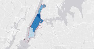
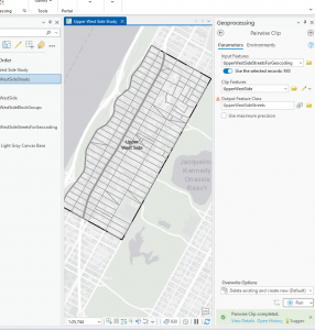
Chapter 6 was another that explored cleaning data up, as the esri book emphasized. We did lots more joins, and I started to get more used to using the tool, but I am not sure how all of this will go when I do not have a book taking me step by step. We also clipped streets to include only the amounts that were within borders, not including the lengths that stretched outside. Below, that is shown.

Overall very frustrating group of chapters, but I suppose that is how you learn.

Montana week 5

Tutorial

Chapter 4


This chapter was all about working with datasets. The first 2 subchapter modules had you implement data sets into the tutorial and started with some dataset management. Later chapters focused on summing data, selecting by certain data fields, and joining data types to find the answers you desire. There was also the introduction of SQL queries which gave some baseline knowledge on how one might code within the SQL language to get the desired data.

 Above is a Maricopa County figure separated by municipalities that was implemented in the first sub module.

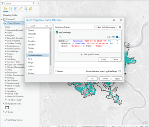
You could switch between the normal easy to read GIS interface and the SQL coding tab to see how the identifiers would be used and written in a SQL query.


Chapter 5

First modules focused on teaching about distortion in a chunk of the world displayed. It illustrates how world maps are less accurate than smaller maps where all features are on a similar geographic plane. Ex: maps of the US are more accurate than maps of the world that have inaccurate representations of Greenland, Antarctica, etc. Many of the modules in this chapter also introduced various coordinate systems to label distinct features at exact locations. There was a lot of work that focused on finding the correct downloaded data in file explorer and implementing it into the GIS. I probably struggled with this chapter the most but I thought the last module was pretty cool and I can see the real world applications for these processes.

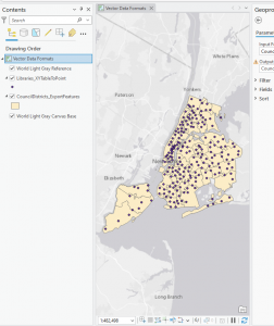
This first map displays libraries spread across New York City.

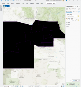
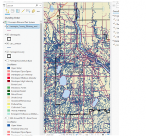
This second one is a map of Hennepin County, Minnesota with elevation contours and bike routes downloaded from the USGS website.

Chapter 6

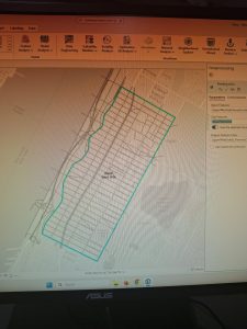
This chapter had us focus on merging and breaking up spatial entities using both the merge tool and dissolving polygons to generalize distinct areas into more regular polygons. It had us use selection tools to find all streets within an area and used the pairwise clip tool to cut off unnecessary street data(pictured below).

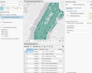
There was a large focus on using geoprocessing tools in this chapter as we did various processes. The image below is a shot of New York fire streets. We can manipulate the data in a way that would be useful to firemen in the city. 

The last module showed similar use by showing the total number of people with disabilities in certain tracts and providing the information of where these tracts fall within fire station territories. I assume that this is useful because firemen have to assume that some people who are disabled(ex: in a wheelchair, can’t get out of bed) may be harder to account for at the scene of a fire or they may need medical assistance themselves.

Week 5 Beard

Week 5:


Chapter 4:

In Chapter 4, we worked with spatial databases and databases in general. This was honestly very difficult, and I did not enjoy it. Having to download the data from the different websites was pretty challenging for me and was not the happiest of my times while doing GIS. This can be a very important thing, though, since some of this data could be important to a specific thing we are looking into, or it could also be something that increases information in our study.

Chapter 5:

In this chapter, we learned how to look at maps using specific locations. Throughout the chapter, we changed coordinates for each of the specific projects and made them show specific areas that were important to search.


Chapter 6:

In this chapter we learned a lot about geoprocessing, which I thought was the easiest chapter out of the 3 we did. This helps us build study areas in our GIS maps where tasks are preformed.  As in this chapter we did a good amount of looking into the Manhattan fire company’s works. We looked at a lot of attribute tables as well which helped point out spatial features, and other important information.

MaBailey Week 5


Chaptwer 4-

There was alot of new information learned in chapter four. We imported data into file geodatabases. Modify attribute tables and fields. Use Python expressions to calculate fields, Join tables. Get an introduction to SQL query criteria. Carry out attribute queries. Point data to polygon summary data.


Chapter 5-

Discussed latitude and longitude coordinates that pinpoint your location precisely on the surface of the earth. we learned about latitude and longitude coordinates and their geographic coordinate system. We learned about map projections, making flat maps from the nearly spherical earth.  This chapter provided some guidelines for choosing a projection.


Chapter 6-

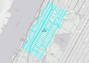
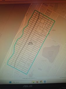
We practiced geoprocessing and set of tools for processing geographic data. We had to use geoprocessing tools to build study areas in a GIS and perform tasks.  Learning how to extract a subset of spatial features from a map using attribute or spatial queries. Processing and prepare layers for emergency management officials in New York City’s Manhattan borough and one of its neighborhoods, the Upper West Side.