Author: zjwhite

Chapter 7).

In this tutorial I practiced the skills of creating and editing GIS features. We learned about the implementation of GPS receivers and applications. We worked with current features as well as to develop new features for the CMU campus of Pittsburgh. 

This first screenshot shows me adding and moving vertex points. The tutorial told me to add 4 to get the right shape, but I added about 6 and still got the same end result, it just took some time. 

I added a feature class and created a point feature for bus stops. I have a screenshot of this:

At the end of tutorial 7, I worked to rotate buildings, and transform polygons. There is a lot that can be done through the edit tab and I think it was super cool to be able to align the polygons of the floor plan with the actual building on the map. The building we worked with was Hamburg Hall in color on the map. I included two sequential screenshots of this process. Overall this chapter went pretty smoothly.

Chapter 8). 

Tutorial 8 was all about geocoding which connects location fields and the rows and columns of the data to the relative fields in feature classes. This maps the data from the data table. This process has many real life applications and uses. There are some limitations to geocoding in that not all matches will be accurate and so a rule-based expert system software is used by ArcGIS pro to facilitate as much correlation and precision as possible. I made sure not to use the World Geocoding Service within ArcGIS pro. 

For the 8-1 your turn exercise, I was able to add a new point to the map via the rematch addresses pane but in the table it was showing coordinates under the match address column whereas the other unmatched records showed as zip codes not coordinates. I can’t seem to find the slight error that is causing this but I still was able to do it. I think maybe the issue was that I corrected the zip code for that last record when I was just supposed to choose an approximate point.  

Once the survey data was geocoded to zip code center points, I symbolized the attendees feature class using graduated symbols, with symbol size increasing as the number of attendees increases:

In 8-2 I worked to geocode the street addresses. I ran into some bumps with the locator tool but I think I figured things out. I built a street locator and set its geocoding option, geocoded attendee data by street address, and then selected minimum candidate and matching scores. For the your turn exercises for 8-2, I found that 872 matched. The tutorial says 873 is supposed to be the number but I don’t think this matters too much. I included a screenshot where you can see the selected records through the attribute and on the map. In order to identify the number of matched records with a minimum score of 90, I used the select by attributes tool to build a query that expressed for the score to be greater than or equal to 90. The results showed a good geocoding performance. 

At the end of chapter 8, I symbolized and produced final geocoding results:

Chapter 9).

In this tutorial we learned the second part of the visualization of spatial data is the analysis of the data. Engaging in spatial analysis helps us to answer profound real life questions raised and displayed by the data. For instance, a map may show patterns or reveal an issue, but the analysis part allows for work towards solutions to that issue or recurring negative trend. The four fundamental spatial analytical methods we explored are buffers, service areas, facility location models, and clustering. I started off by using buffers for the purpose of proximity analysis. A buffer is simply a polygon that encompasses map features of a feature class. 

Here is a screenshot of the first your turn exercise in 9-1. We created a buffer of the pools feature class, particularly a one mile buffer. Then I performed some analysis, calculating the number and percentage of youths within that distance. I found that 42,548 youths are within that distance. About 87 percent of all youths in the city are close to a pool. 

This next screenshot is from tutorial 9-3 in which I created multiple-ring service-area polygons, spatially joined service areas and pool tags, calculated pool use statistics for service areas, and finally created a scatter plot.  I had some issues with the spatial join tool but I got through things it just took much longer than expected. 

For the very last part of 9-3, involving fitting a curve to the gravity model data points, I was able to open the excel spreadsheet but the beta values were already entered. Thus, the resulting average absolute error values were already there as well. And I’m not sure if we were supposed to just take a look at this stuff or actually do something. It seemed like we were just exploring the spreadsheet and noting those things so I moved on. 

For the 9-4 tutorial your turn exercise, I was able to do the first model run and create the first map but when I tried to do the second model run I kept getting Solve errors. I was able to work with using Network Analyst to locate facilities and see what this looks like, but when I kept getting errors for the second model I tried to figure out the issue but it kept occurring. I included a screenshot of what I produced and I learned that this sort of map is used for visualization. You can see the lines and essentially the lines show the demand relationship between pools and block centroids.

For the your turn exercise of tutorial 9-5, I was able to run the summary statistics tool and create the table with the mean values, but there were a few rows that were in different places then what arcGIS pro showed. I got all the exact same values, things were just in varying positions. Below is my work from 9-5 with performing a cluster analysis. 

Chapter 4).

In this chapter we actively worked with geodatabases through which data can be stored, analyzed, and more. In specific terms we worked on storing feature classes and raster data. Data tables can be related and joined. Something important to remember is that attribute, field, variable, and column are interchangeable names for the columns of data tables, and record, row, and observation are interchangeable names for the rows in a data table. We worked to use a shapefile which is a spatial data format for a single point, line, or polygon layer. I included a screenshot of my work converting a shapefile to a feature class and the tools used. 

In 4-2 we worked on deleting, creating, and modifying attributes as a crucial part of processing and display of our data. I included a screenshot of modifying attribute tables, particularly delete unneeded columns. As you can see in the table, only the needed five attributes remain at the top. 

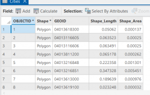
For 4-2, step 4, there was only one basemap showing activated in the contents pane, not two of them. I included the your turn work for 4-2 in which I worked to modify the attribute table first through working in the fields section of data design. I also modified an alias, particularly the name field and changed it to the alias of city. This is shown in my screenshot. 

I extracted substring fields and concatenating string fields, calculating attribute fields, and sorting things around via the MaricopaTracts attribute table. There is a lot that goes on here and while I got through it no problem I don’t think I’ll be able to reproduce all of the steps right away. I think it is however super cool how we can extract parts of text strings and reassemble them into a new text field and calculate a range of values through precise expression inputs. In 4-3, I practiced carrying out attribute queries. The main function here is that essentially an attribute query selects attribute data rows and spatial features based on attribute values. There are simple and compound SQL criteria. 

In 4-3, step 7 of the query a subset of crime types using OR connectors and parentheses section: All of my dots were staying that light sky blue color on the map even though I had burglaries as green and robberies symbolized correctly with a dark red. I had no problem with the subsequent your turn exercise in which I edited the query and symbolized the burglaries with a dark red. For the last my turn exercise in tutorial 4 in section 4-6, I tried to symbolize crimes by giving each crime a different symbol but it didn’t go too well I think because there was a null class that was showing. The map didn’t look visually appealing and was hard to read as the null symbol was covering everything. 

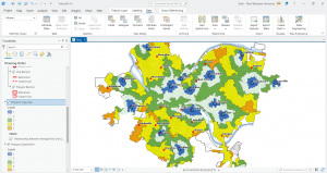
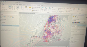
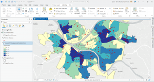
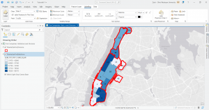
I included a screenshot of the your turn exercise for 4-4 in which I created a choropleth map using graduated colors. The reason the red dots are still present is because I was yet to turn off the crime offenses layer.

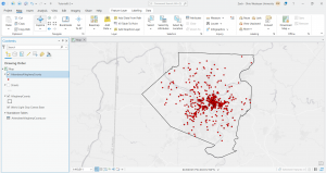
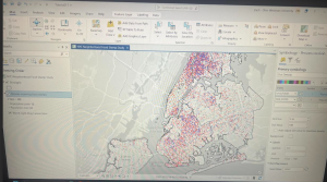
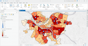
Graduated symbols for the next your turn exercise for the following tutorial 4-5 is below. I created a point layer with the output features class of BurglariesByNeighborhoodPoints and then symbolized things. 

Chapter 5).

In the chapter five tutorial we explored sources of spatial data. We took a look into ArcGIS Living Atlas and both a US federal and a local data source. We worked with map projections and coordinate systems. I was unable to participate in some of the work in this tutorial as I am a strong believer in a flat Earth. Some really cool and meaningful questions come up in this chapter.   

I was unable to do tutorial 5-2 step 3 of the section called set projected coordinate systems for the United States. I tried clicking the USA Contiguous Albers Equal Area Conic about three or four times and every time it would freeze my ArcGIS Pro and I would have to fully shutdown my computer to get anything to load again. I simply proceeded to the your turn exercise that followed. When I tried implementing the different projections to the US map the same thing occurred. Given this 5-2 tutorial was very short and I understood the main point, I just moved on. 

In 5-3, I added a new layer to set a map’s coordinate system and then I added a layer that uses geographic coordinates. I include a screenshot of this and the symbology work with the tracts and multiplies layers is also shown. 

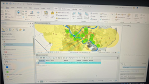
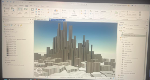
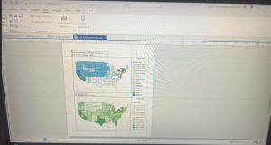
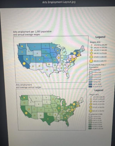
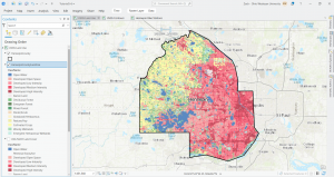
Tutorial 5-5 was super tough to get through and there were a lot of steps that required you to memorize and apply past steps and so I had to go back and remind myself but I got through it and the end result felt nice. As you can see in the screenshots below I joined data and created a choropleth map. I explored things by turning layers on and off. 

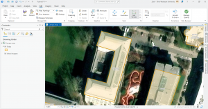
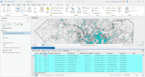
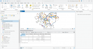
My next photo is from 5-6 where I was downloading geospatial data and extracting raster features for Hennepin County. There were a lot of technicalities and difficulties here too but with some time and going back to certain things for assistance, I was able to pull it through. 

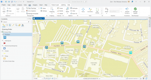
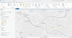
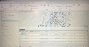
For the very last part of tutorial 5-6, in which I attempted to download local data from a public agency hub, there was NO option for bicycle count stations (step 2). I tried downloading the data for the Hennepin County Bike and Pedestrian System but this did not work well. I’ve included a screenshot of the results when I tried to access the data for bicycle count stations via the agency hub.

Chapter 6).

In chapter 6 we furthered our understanding of geoprocessing. We used geoprocessing in past chapters but we built on its capacity here. Something significant we did is we used intersect, union, and tabulate Intersection tools to combine features and attribute tables for geoprocessing.

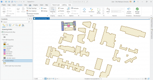
I included a screenshot for the first your turn exercise where I dissolved fire companies to create battalions and divisions.

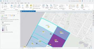
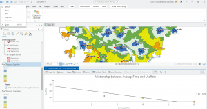
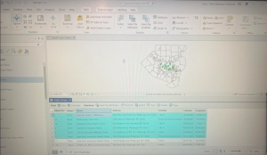
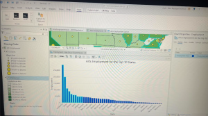
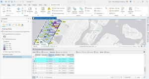
At the end in tutorial 6-7, I studied the usage of the tabulate intersection tool. I worked with some interesting maps that relate to real world matters through exploring tracts and fire company polygons. I then used the used tabulate intersection to apportion the population of persons with disabilities to fire companies. The screenshot shows a zoom to fire company 76 and the next displays the DisabledPersonsPerFireCompany table that I created after running the tool. The last thing I did in this tutorial was use the summary statistics tool to create a TotalDisabledPersonsPerFireCompany table. I like how these processes and the work we practice here can and are used in the real world for planning purposes or joined to fire companies for map creation. Overall, I am feeling a bit more comfortable with things, but there is still a decent amount of confusion and I consistently have to refer back to previous steps and chapters for support.

 

Start work week 5 for final assignment:

Steps 1 and 2:

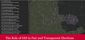
Zip code Data Layer:

In 2003, the zipcodes for Delaware County were reworked. When evaluating zip codes, there is collaboration between the Census Bureau, the United States Postal Service, and the U.S. Treasurer’s office. It says this data set is updated as needed but does not give specifics. It says it is published monthly, I guess indicating that any changes will only be seen on a monthly basis. 

Street Centerline Data Layer:

Ran by the The State of Ohio Location Based Response System. This is something I’ve never heard of before. Focuses on the center of pavement of both public and private roads. Some main functions are to assist emergency response teams, manage disasters, and even geocoding which we learned about this week. All fields are updated daily but 3-D fields are updated once a year. 

Recorded Document Data Layer. 

Involves record documents like annexations, vacations, or miscellaneous documents within the county. It says the data points show record documents within the county recorder’s plat books, cabinet/slides and instruments records. Not too familiar with these terms but above all, I have no idea what a plat book is. Can be helpful for locating lost or miscellaneous county documents. 

Survey Data Layer:

Point coverage that shows surveys of the land within the county. The recorder’s office and map department manage survey points. Up to May 2004, GIS staff scanned the surveys but after 2004 the map department took over. Important for providing legal and authorized info about land features and boundaries. 

GPS Data Layer:

GPS monuments in the ground or survey benchmark devices from 1991 and 1997. Why does it just include those established during these two years? I’m guessing this can be used for location data and important planning, management, and emergency services. Geographic patterns through GIS makes GIS even more powerful. I remember mentioning this in my post during week one I think it was.  

Parcel Data Layer:

Includes polygons of the official boundary lines that define a specific plot of land within a public record. Public record geometries are managed by the DelCo auditor’s GIS office. Any changes made are managed by the county recorder’s office. Important for providing detailed information on land use, land ownership, and I read land value as well. 

Subdivision Data Layer:

Managed by the county recorder’s office. Subdivisions mean that a large plot of land was divided into smaller parcels. The summary mentions condos as for example, a condo project can be a type of subdivision. Critical for urban planning, real estate, and governance at large. 

School District Data Layer:

Shows all school districts within the county. Important for data-centered decision making to improve education and schooling circumstances, thus bettering students. I think this data layer is important for resource allocation and makes that distribution more equitable. Facilities of schools can also be managed effectively with this data. 

Tax District Data Layer:

Shows all tax districts managed by the county auditor real estate office. Mentions that data is dissolved on the tax district code I guess meaning that data for a certain geographic area is done with or being merged due to an issue with whoever originally created the code. Important for municipal finance like billing and collection as well as property tax assessment. Can also be used for community planning and helping locals maybe understand what services they can get and whatnot. 

Township Data Layer:

This layer shows the 19 townships within DelCo. It shows very clear legal boundaries. Important for tracking and defining property rights especially if there is a large land tract or agricultural tracts. Also important for understanding how the township plays into the administrative duties of local, state and federal levels of governance. Looking at township data can be super useful for infrastructure projects and development.

Annexation Data Layer:

Data all the way back from 1853 to the current day that shows the county’s annexations and conforming boundaries. Important for showing how boundaries change and helps with many government functions. Super significant for census and demographic data and the Census Bureau relies heavily on this data layer.  

Address Point Data Layer:

Shows all certified addresses within the county and shows the location of the building’s centroid. Very helpful for reporting accidents or emergency situations. Has the capacity to reverse geocode a set of coordinates to provide the closest address which is highly useful for emergency response teams. I never really thought about this reverse geocoding but it is something that definitely occurs and is vital for say the police to find a suspect of the location of a crime. 

PLSS Data Layer:

Includes the public land survey system polygons for the US Military and the Virginia Military Survey Districts of the county. I’m not familiar with these US Military the Virginia Military Survey Districts but I can assume the PLSS layer is crucial for government records and legal descriptions for like when property is bought or sold per say. I read that in some cases historical land division and ownership regulations of guidelines still impact modern day property lines and so forth. 

Building Outline 2023 Data Layer:

Updated in 2023, this layer includes all the building outlines for all structures in the county. I think that this accurate representation of every structure is significant in general but I can see this layer being used a lot for urban planning considering the rise of urbanization as well as maybe things like smart cities or eco friendly cities. 

Condo Data Layer:

All of the condominium polygons for the county. As mentioned earlier in the subdivision data layer section, a condominium project is an example of a subdivision so this is kind of redundant unless condos are something incredible and it gives insight into this. I understand if this is used to focus strictly on condos but I don’t see why it can’t serve the same purpose in the subdivisions layer unless I am missing something here.

Farm Lot Data Layer:

Again there is this involvement of the US Military and the Virginia Military Survey Districts of the county for this layer that shows all the farms. Critical for modern agriculture and land management, helpful for maybe the efficiency of operations. Can help farmers and can help improve land and resource management that helps the economy and everyone. 

Precincts Data Layer:

Shows all of the precincts in the county. Helped run by the county board of elections. Helps to show and analyze voting patterns. This is important overall for supporting informed decision making in all election fields especially in the election and voting climate we live in today. Displays voting behavior and demographics. 

Delaware County E911 Data Layer:

This is a major one used to contribute to the pursuit of accurate and efficient emergency responses. Provides emergency dispatchers with emergency location and gives these first responders significant geographic data. The summary of the layers describes that it gives a spatially accurate representation of all certified addresses so these 911 events are handled smoothly. 

Original Township Data Layer:

Not much summary for this one but I guess it is used as like a legally-binding record for land ownership and administration and things like that. The layer description mentions that original boundaries of the county townships are shown. There is an indication that this layer is significant because these boundaries came before tax district changes modified their shapes and so forth. 

Dedicated ROW Data Layer:

This layer shows all lines classified as right – of – way in the county. This layer maps and helps to manage areas of land use like transportation and utilities. This is important because while a probity wonder may own a part of the land, the public has the right to use the land for a certain purpose like I mentioned before. I can see how this can create conflict with landowners or homeowners and such. 

Building Outline 2021 Data Layer:

Updated in 2021, this layer shows the outlines for all structures in the county. I already read about the building outline 2023 layer and so I’m confused on why this earlier layer would be used. Especially for infrastructure and buildings, the most recent and updated outlines are utilized. I can see if this is used to track changes, or comparing historical data maybe when managing a complex project or something. 

Map Sheet Data Layer:

When I first heard map sheets I thought of a single standalone printed map. What I understand is that it can be a single map in a larger series that way a data can separate different types of data like roads and rivers. I guys if you have different management sheets you can better see things rather than having everything thrown into one image or whatever. 

Hydrology Data Layer:

Shows all major waterways within DelCo. Enhanced in the past with LIDAR based data. This must be incredibly useful for spatially representing all water related features. This can then be used to manage and protect both man made water systems and natural bodies of water as the more common of the two here in DelCo and probably everywhere. 

ROW Data Layer:

Again, this consists of all lines that are designated as right – of – way in the county. Why is this different from the one I already read about called the designated ROW data layer. Does one of them involve future planning and considerations of ROW. Does one of them involve the actual and current ROW classifications or regulations? I’ve never heard of ROW and so I’m a bit confused. 

Address Points DXF Data Layer:

Shows the accurate positions of addresses within a given parcel within the county. The state of Ohio and DelCo worked collectively to formulate this layer. Again, this is another layer as to why this is different from the original address points data layer I read about. I looked into the DXF in the name which stands for Drawing Exchange Format. It says this is the file format used to distribute GIS data to people like surveyors and just the general public. 

2024 Aerial Imagery Data Layer:

This layer includes the 2024 3in Aerial Imagery. This imagery was recorded in 2024 as it says drones or whatnot were flown then in the spring time. This is so very useful for enhancing the visual content that GIS works with and as a result that those who work with GIS work with. This data can allow for better mapping and visualization of the Earth’s surface for a range of applications. 

2022 Leaf – On Imagery SID File Data Layer:

This layer shows imagery with a 12in resolution from the year 2022. There isn’t much summary but I can infer this is aerial or satellite images taken during like a growing season where trees and things have leaves. I guess the timing of this is super important for certain functions and analysis to be done. 

Street Centerlines DXF Data Layer:

The  Drawing Exchange Format showing the center of pavement of public and private roads in the county. It says that address range data which is like a span collection of addresses represented by a value pertaining to one side of the road versus the other. It says this data was collected by field observation of address locations that do exhaust and by adding or maybe even changing addresses through building permit info. 

Building Outlines DXF Data Layer:

The Drawing Exchange Format for all outlines of structures in the county. A summary was not loading and I was having trouble opening things. 

Delaware County Contours Data Layer:

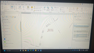
This is a data layer from 2018 of two foot contours. These two foot contours connect points of equal elevation with a distance up and down of two feet between the lines. I wonder if LIDAR was or is used. This allows for visualization of things like elevation and terrain features. Terrain features with a specific political or whatever boundary can be visualized through this layer.

2021 Imagery SID File Data Layer:

2021 image data. I’m not sure if this pertains to general aerial imagery or leaf on imagery. I was confused on this SID acronym but I looked into it and it said that SID is a Multi-resolution Seamless Image Database.

Sidenote: I was unable to access some of the data layers whatsoever. I tried multiple times to reload things but the system would not work. I had only a couple left to read and review, not sure why these final layers malfunctioned. I read the summary from the main page and got what I could out of them without clicking on them. This occurred for only two or three layers. 

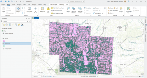
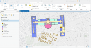
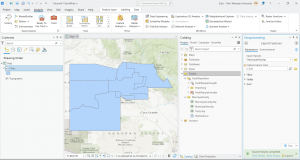
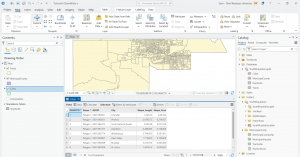
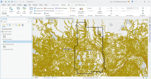
Steps 4, 5, and 6:

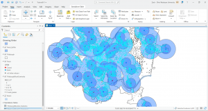
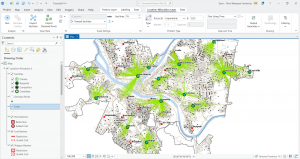
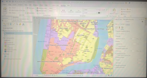
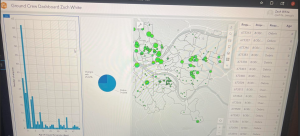
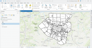
I downloaded these three data sets: Parcel, Street Centerline, and Hydrology. I then created a map that shows all three but I have no idea if I did it right. I was having trouble extracting the files and getting them to show up as I opened a new project. I bypassed that by opening a map on the ArcGIS pro home screen and then working through things. Here is a screenshot. 

Chapter 4).

Mapping density is crucial for identifying patterns relative to where features are concentrated. Concentrated areas of crime for example will need action by law enforcement. Mapping density is useful for mapping areas (census tracts or counties) of different sizes and showing patterns rather than details about individual features. In order to map density, we can either shade defined areas based on a density value or create a density surface. Generally features of GIS are mapped using a density surface. The other thing we can do is map already summarized data by defined areas like administrative boundaries. We can either map density features or feature values that we talked about last week. A feature value goes beyond just the feature location like the number of employees at each business. Density by defined summarized area does not show actual feature locations but rather represents a specific number of features. Density = # of features / area of polygon. We may need to use a conversion factor to keep units consistent. On the other hand, the GIS creates a density surface as a raster layer and can be locations or linear features like roads. Map density surface if you have individual features or sample points. Density by defined area seems simpler but density surface mapping looks better but is more complex to do. ArcGIS imposes density by defined area on the maps by shading. For a dot density map, we map each area or dot based on a total count or amount. Two different size census tracts with the same population would be the same color on a shaded map but a dot density map shows that the smaller tract has a higher density with the same number of dots in a smaller space. Dot maps are not calculated density values but the actual total numbers or values for each area. The four parameters of cell size, search radius, calculation method, and units are important considerations for calculating density values. I’m not too comfortable with calculating cell size and density converse and so I’ll definitely have to refer back to the book if we have to do this. A tip to remember is to use a value for units that reflect what features we are mapping Square meters for plants or trees and square miles for businesses. Another cool thing is that we can create a density surface using center points from data summarized by defined areas. When displaying a density surface, we employ graduated colors by creating custom class ranges or allow the GIS to do this through a standard classification scheme. Overall, the patterns of the map depend on the creation of the density surface and its parameters. 

Chapter 5).

Finding what’s inside allows us to evaluate if something occurs within an area or identify comparable information for different/multiple areas. Comparison here is important because it can be crucial in some cases to know what surrounding areas have within them or not. In order to find what’s inside we can either draw or utilize area boundaries. The number of areas and the types of features in those areas are fundamental. A grouping of zipcodes would be several areas combined. Identify each area with a name like the name of the watershed for example. We can use the GIS to get a list, count, or summary of the features within an area. We can include features that fall completely inside (for amounts), partially inside (for lists and counts), or the portion of each feature inside the area. The overlaying the areas and features approach seems good by showing what features are inside and summary details but takes longer to process. If you’re overlaying an area on data that’s summarized by area, we should make sure the summarized areas fall completely inside. This is good to do with multiple areas or single areas that need summaries of continuous data, or discrete features including only the portion inside the area. To distinguish areas when actually making the map, label them and or draw in a different shade. When selecting features inside an area and using the results it is good to know what a frequency is. A frequency is the number of features with a given value or range of values. A bar chart can be shown for numbers and a pier chart for proportions of a whole or percentages. The summary of a numeric attribute of a feature can be a sum, average, median, or standard deviation. A sidenote is that we can show what is inside the area only but it is good to show the features outside of the area as well for contextual information. I like the look of showing features inside the area with a darker color and features outside with a lighter shade of that same color. When overlaying areas with continuous categories or classes the GIS will generally select the modeling whether it be vector or raster methods based on the data we have.  Pay attention to slivers which are very small areas that are there or emerge after overlay. Remove them at first or have the GIS remove after mapping. Sometimes Raster overlay is the default or the GIS converts it to raster because it is simpler. The GIS also creates a table to analyze the results of the overlay for the raster method. Geez vector overlay seems much more difficult.  

Chapter 6).

Finding what’s nearby is super good for considering events in an area, finding the area served by something, or the features affected by something (homes impacted by flooding). What occurs within set distance or traveling ranges is critical for many uses of GIS. In order to find and evaluate what’s nearby, we can measure straight line distance, measure distance or cost over a network, or measure cost over a surface. In cases where no movement between the source and surrounding features, measure using straight-line distance. If there is movement, travel can be measured over a geometric network like a street or over land. Finding what’s nearby can also be done by measuring costs which include time, money and or effort. This relevance of the curvature of the Earth comes into play here again in that calculating distance under the conditions of a flat Earth uses the planar model while doing this under the conditions of a spherical Earth uses the geodesic model. This distortion only occurs again when the area is large but for small areas of interest it doesn’t apply and planar modeling can be done. It is important to consider whether we will need a list, count or summary, and how many distance or cost ranges are needed. If we want to know how many streets are within 1, 2, and 3 miles of a fire station, we can use inclusive rings or distinct bands. 

Chapter 1). 

GIS analysis is a process for investigating geographic patterns in data and interpreting the relationships between associated features. At the core of GIS analysis is a similar starting point to analysis in all fields. The book says the first step is to frame a question. In scientific research, we have research questions. Really when doing any sort of report, essay, project, we have a research question. In politics and government I learned a lot about framing which is the gathering or presentation of information under a specific context in an effort to dictate how it is understood. I think the critical point about this step is to develop your question in as much specificity as possible, that way you have a direct approach to the analysis, a concrete method to go about, and a particular plan for presenting the results. This is something we have learned generally here at OWU overall in terms of limiting the generality of a research question and instead making it as precise as possible. Another super important thing to consider at this stage is the target audience and the context of usage. For the understanding your data stage, I think that it is important to recognize that this goes beyond just the header of knowing your features but also includes the capacity to build new data from existing sets. This taps into the fact that GIS can be used not only to analyze current geographic patterns and data, but also to construct new ones. For the methods, a key point is that how the data will be used fundamentally influences how you obtain and formulate that data. Once a method is chosen, I think it is super helpful to know that you can compare and contrast different analyses in order to proceed with the information that is most fitting in terms of presentation and accuracy at large. I think these preliminary steps and considerations will be exceptionally useful in making the process overall more straightforward. Moving on to geographic features I think that the distinction between continuous and discrete features is significant in that discrete features represent an actual value and a specific location like businesses represented by the number of employees. On the other hand, continuous variables have a range and can be measured at any given location and encompass the entire mapping space like temperature. In context, there may be a business with a large number of employees and then an area with no business at all. And so with these discrete features there are gaps involved. Something important to remember with continuous information is that it can be spaced regularly or irregularly. For example atmospheric pressure readings for environmental monitoring are recorded at the same time every hour per se and so there are these set intervals at play. Continuous data can also be irregularly spaced which essentially means there is no uniform interval of spacing/measurement involved. I was a bit confused by the term interpolation but from my understanding it uses discrete data and known points to approximate values for potentially unknown locations involved with continuous data. The point then is to formulate a continuous mapping space which can be essential for mapping some continuous phenomena. Another main distinction I took away from the discussion of continuous and discrete data is that boundaries are modeled and interpreted differently showing degrees of similarity for continuous data and showing legal borders if you will for discrete data. While features can also be summarized by area, oftentimes data comes summarized by area (data found within set boundaries). I think it’s cool that we can perform basic statistics to summarize any additional data by area, then merging the data tables and mapping to identify connections. Moving on to representing geographic features, in my head I aim to think of the vector model as the x, y coordinate model. This is based on the rows of data tables. Locations get coordinates, lines get coordinate pairs and areas get borders. The raster model contains features that are shown by cells spaced or layered across the map in a continuous space. Discrete features and data summarized by are are generally modeled by vector. Continuous variables are modeled by vector and raster but continuous numerical values are shown using raster modeling. Due to the map projection translation process, the distortion of features is something to consider when mapping larger areas. For the types of attribute values a cool thing I learned is that we can assign ranks based off of other attribute features. Rasta modeling comes into play here for this multi criteria ranking and multi layer data mapping. Ranks put features in order when values are hard to quantity like if I want to look at the scenic or recreational value of a body of water through a city. The main point for counts and amounts is that a count is the total number of forests on a map whereas an amount can be the number of trees within a forest. Ratios are good for showing evenness in terms of the distribution of features. The number of people in an area divided by the number of households is the average number of people per household. Categories and ranks are discrete whereas counts, amounts, and ratios are continuous. For doing the selecting, calculating, and summarizing components of working with data tables, I think I get most of it, I will just definitely need some hands-on practice to make sure I do.  

Question:

Is there a way to manage the distortion of features when mapping larger areas or is it just something to consider when evaluating the map and when presenting?

Chapter 2).

Mapping helps us understand where things are but also much more. Through the patterns of placement that can be devised, we gain insight on why things are where they are. In this sense, it’s more beneficial to look at the distribution of features, the full story rather than individual features or the single story. Like we learned from Schuurman, GIS is used by many different types of people for a vast range of purposes and mapping where things are can serve a totally different role for a police officer than for an ecologist. When thinking about what to map, it is helpful to use symbol types based on what features you are looking at and how the map of those features will be utilized. We can map different types of features to see if there is any overlap. Information depth can vary based on the audience the map is being shown to and the medium through which the map will be presented. When preparing the data to be mapped the assigning of geographic coordinates is essential. Data from any GIS database already has assigned coordinates but if we bring data in from any outside source then we must include a street name or latiutude/longitude to register with GIS to internalize and dispel coordinates for us. Major types and subtypes of features can be obtained from already stored information or created by adding a category in the data table. When actually making the map we can map single types of features or show multiple features by category values. Single type features get the same symbol when mapped which often does still reveal patterns. We can map all features or a subset of features to seek more intricate patterns for individual locations. A main point I got here is that it is good to show all types but if you want to do a subset then just highlight that and make the other types a lighter color shade. Another tip I took away is that using different colors or symbols for each category value of the feature is good for displaying the hierarchy of features and being able to distinguish the types of features. Features can also belong to more than one category and we can show that. There are burglaries overall, then types of burglaries, but also things like the type of buildings entered for a burglary. NO MORE than 7 categories, break it up and do a side by side evaluation. When grouping categories we can assign one record a code for its general category and a code for its detailed category in the database. For locations, use colors to distinguish categories and for linear features use different widths or patterns or lines. Displaying reference features like landmarks or major waterways can be helpful for serving a representative audience in terms of being able to recognize and relate to the map. I learned that a useful tool is to choose simple monochrome base maps of ArcGIS for this mapping reference features component. In terms of analyzing geographic patterns, scale has a big impact and so zooming in and out may be needed. Clustered, uniform, and random are three core types of distributions to look out for. 

Question:

For our work in this class, will base maps be used most of the time, sometimes, or will we always have to include reference features?

Will there be cases where we are obligated to bring in data from outside sources, not GIS data bases, then having to give GIS a basis to formulate coordinates for us? Or will we mostly be dealing with data from ArcGIS?

Chapter 3).

Mapping features based on a quantity associated with each feature adds an additional layer of helpful information. This is essential for thinking about these overarching goals of finding places that align with what we are looking for or identifying relationships between places. Similar to the example the books describes, I thought of one in that mapping crime based on where crime has occurred gives us an understanding of crime overall but mapping crime based on the number of crimes committed at each location give a much more accurate depiction of the levels and frequency of crime. If crime has occurred once or twice in one area, but has occurred 100 times in another area, those details on where crime is concentrated is much more useful.  To represent quantity, location and linear features are represented with graduated symbols while areas are typically shaded to show quantities. Continuous features as defined areas can be shown through graduated colors while continuous surfaces are shown using graduated colors, contours, or a 3-D view. Examples of areas can be zipcodes or watersheds. In terms of further understanding quantities a count is the number of people in a census tract whereas an amount is the number of 30-45 year olds per se. When summarizing an area, it is best to use ratios as areas differ in size and using ratios will best represent the distribution of features. We also need to be aware that we are working with the right ratio. Average is the most common type of ratio and best fitted when comparing areas with a disproportionate amount of features. A little reminder is that when calculating averages we divide quantities that use different measures and when doing proportions we use the same measures. Density as another type of ratio is used to show concentration of features calculated by dicing a value by the area of the feature to get a value per unit of area. When mapping quantities there is this overarching tradeoff that exists in between displaying the data values most accurately and generalizing them to visualize patterns. Counts, amounts, and ratios are typically generalized into classes. The four most common standard classification schemes are natural breaks, quantile, equal interval, and standard deviation. A good tool to use is to plot the values on a chart to understand the distribution and then select a classification scheme. I am a bit confused on how to do these classification schemes and the making of the charts to figure out distributions but I think with some practice that will be fine. I get the general idea of each classification scheme but it will definitely take some practice to be able to work through these. When working through this, it is good to remember to use natural breaks for uneven data and for even data use equal interval or standard deviation. Use of quantile shows relative differences between features. Something I took away as a reminder when juggling all of this is that ArcGIS allows us to easily and quickly change classes, symbols, and so forth. This is helpful when trying to explore the data and seek out patterns. Another pointer is to be aware of outliers that can either be eros is the data set or abnormalities from a small data size. Outliers can be marked as insufficient data as a last resort. When managing the number of classes, changing this will bring out patterns more or make them less clear. In order to make the map most understandable and readable, we can work with the legend and round out min/max values. We may also have to manually go in and edit the class values once the GIS has defined them for us. This goes especially for natural breaks classifications. We can also change the numbed values to high or low if there are meaningless decimals making the map harder to read. When making maps, keep them simple and show only information that effectively displays the patterns. When using graduated colors use darker shades to indicate higher class values. When using graduated symbols the main takeaway is to use symbols that show patterns without obscuring feature locations. I think using charts is hard to read and graduated colors are easier to read and show the details. Employing graduate charts makes this a bit easier to read and shows the relative sizes of each feature. I like this a bit more. For 3D perspective views, I am a bit confused on how to combine the z factor with light source. There is a lot of description on how this is done but I think it will be helpful to see it done or try to actually do it. 

Question:

Do we need to know the internal operations of GIS when performing certain processes that give us the classifications schemes or values that we are looking for? There is some discussion on what the GIS is doing in detail and so I am wondering if that is something we need to understand or pay attention to.

My name is Zach White. I am an environmental studies major with a minor in Spanish and politics and government. I love basketball, fishing, and music. 

 

I took the GEOG 291 quiz and it went smoothly. I wasn’t too particularly pumped about taking GIS but that was mostly likely in part due to the lack of involvement or familiarity I’ve had with it thus far. Coming in with little to no exposure, I would definitely not have thought that specialty doctors use GIS to discover or explore disease. If anything, I’ve kind of correlated it in my mind to GPS up until last year lol. Turns out GIS and GPS are indeed different. I like that the reading doesn’t target a technically minded audience but rather a more representative audience. This is helpful because as Schuurman points out, ordinary people use or are impacted by GIS daily without even knowing it’s at play. 

When a problem emerges, it is fundamental to consider both the social context of the issue and the historical significance. It is critical to look into this because problems develop, go away, and reemerge through history, and problems are tightly connected to the societal conditions of when that problem persists. I learned this in my sociology course today and so I can appreciate the discussion of the identity of GIS and its pervasive relevance now in comparison to the historical implications. This also reminded me of the interdisciplinary nature of our liberal arts education through a GIS course in which different types of people use GIS in completely different ways with distinctive objectives. The history of how overlay became spatial analysis is intriguing. It is this historical advancement of technology that bolstered this transition and that continues to have an effect today.

I was a bit confused at the start of the reading when Schuurman explained that Geographers kind of opposed GIS. It became much more clear after reading about the history of GIS and how the analysis side of it differs from the physically visual and geographically based creations that are maps. Cartographers were familiar with their maps and not the information extraction and more detailed exploration that GIS offered. Maybe this is why I was not jumping out of my seat to learn GIS.  

The following discussion of the visuality of GIS kind of contradicts why geographers may have opposed it, highlighting that GIS actually enhances this visual component by making this newer development more meaningful and more widely accessible. I like this because I definitely fall into the category of those who gain more information through visual arrangements than from a table with numbers or text. This idea that GIS goes beyond traditional analysis through its visuality is something that has made my interest in the course overall go up a bit. 

The conversation of GIS as a software and GIS as a science is interesting. I never thought of the idea of a GIScientist but this seems cool. From my understanding, a GIScientist is more focused on the output and the evaluation of GIS input work while still considering the conditions of input and if that serves the output in one way or another. Through the connections that emerge through the inputs, my understanding of the main point for GIScience is that this process can then be justified and or contradicted based on its means of implementation. Through the investigation of input relationships, there then is this component of presentation that applies to GIScientists and researchers for which the diffusion of accessibly interpreted results is the goal. I think the increasing understanding of the importance of social influence on GIScience and GISsystems is vital in a world that is progressively dictated by the current society and its direction. 

GIS application 1:

I’ve always been interested in sharks and their behavior as the apex predator of the oceans. I’ve also had experience tagging sharks when I was younger and I did research on the shark sanctuary conflict in the Maldives last year. There are various sites that show the movement of sharks along with other ocean ecosystem indicator species. GPS is used in terms of pinpointing shark locations and data is transmitted from the tag to a satellite. GIS is also used and like we read in the reading GPS and GIS are utilized by combining GPS with GIS. I found this one site  that centers a non profit working to expel data that has been unattained or unexplored in an effort to assist scientists and other sectors like education and policymaking. 

Tracking, M.-W. (n.d.). Ocearch Shark tracker. Retrieved from https://www.ocearch.org/tracker/

While in this first display, GPS is largely at play, the next depiction from the same organization shows more clearly their implementation of GIS to go beyond a location and explore spatial patterns and relationships across layers:

https://www.ocearch.org/tracker/

GIS application 2:

For my interest in politics and government I wanted to look into the role of GIS in politics, particularly elections. I found a really cool study done by Harvard University that investigated how GIS can assist in understanding the conditions of elections and how things like jurisdictional complexities impact elections and the people at the core of these processes.  

The role of GIS in Fair and transparent elections: Data-Smart City Solutions. (n.d.). Retrieved from https://datasmart.hks.harvard.edu/role-gis-fair-and-transparent-elections