Week 4 – Savannah Domenech

Getting to Know ArcGIS Chapter 1

Notes and Comments:

  • GIS is composed of five interacting parts: hardware, software, data, procedures, and people
  • Spatial data is information that represents real-world locations and the shapes of features at those locations and the relationships between them
  • GIS, like mentioned in the Mitchell book, is a visual, quantitative, and analytic tool
  • Geoprocessing is the manipulation of spatial data
  • Open data allows anyone to get authoritative data and information. ArcGIS Hub is a way the public can freely access maps and data
  • I find the concept of open data fascinating as one of the goals of it the book mentions is the ability to get right to problem-solving. We have so much data, especially in research papers, but I feel that it is hard to take action
  • It’s good to keep in mind that ArcGIS Desktop is a suite and not just confined to ArcMap and that ArcGIS Pro is part of the ArcGIS Desktop suite

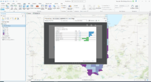
Exercise Notes and Screenshots:

  • I couldn’t find the outline toggle in step 12 of Configure the map symbology so I skipped it; I do not believe it made a difference
  • Despite this book being pretty new, the names for a bunch of things are somewhat different than the book records them to be

Getting to Know ArcGIS Chapter 2

Notes:

  • ArcPro and ArcOnline communicate with each other much better than ArcMap and ArcOnline as ArcPro allows you to sign in
  • ArcPro projects can contain multiple maps, geodatabases, folder connections, layer files, task lists, models, toolboxes, and more
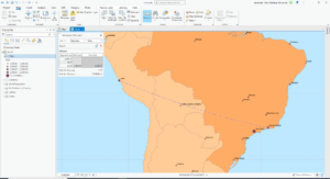
  • The world symbol next to the “Explore” tool is the full extent button
  • The feature layer ribbon is activated any time a layer in the contents sidebar is selected
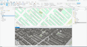
  • Extrusion is the process of stretching flat 2D features vertically so they appear 3D
  • To package a map there must be a description in the map’s metadata

Exercise Questions and Screenshots:

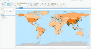
  • (Modify map contents 5) PM concentrations are highest in Africa
  • (Examine the contextual ribbon 2) If you close the content pane, go to “View” and click “Contents.” The Geoprocessing tool is next to the “Contents” button
  • (Examine feature attributes 4) Shanghai, China has the largest population
  • (Create a 3D scene) The height of the tallest building is 339.76


Getting to Know ArcGIS Chapter 3

Notes and Comments:

  • Definition queries make certain features or areas invisible but they do not get rid of them
  • To subset from a data set you can use a definition query, the clip feature, or the select and export feature
  • Joining the join table to the attribute table requires that the attribute type is the same (e.g. text joins to text)
  • You cannot have spaces or more than 10 characters in the field heading in the attribute table
  • Spatial join allows you to join data based on location. You combine the target and the join layer into a new output layer
  • I can follow along easy enough but if you told me to do this on my own I would be clueless

Questions and Screenshots:

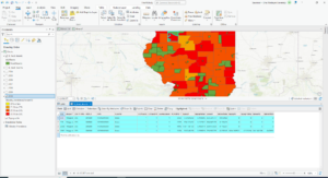
  • (Add data to project 5 part 1) The field name that indicates which state the county is in is STATE_NAME
  • (Add data to project 5 part 2) The number of Wayne county residents between ages 22-29 is 10,575
  • (Join data tables 3) Six years of data are represented
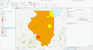
  • (Overlay additional data 1) No, I do not see a clear correlation between income and 2010 obesity rates. While many counties with high obesity rates have lower incomes a moderate number of counties with moderate to high incomes also have high obesity rates
  • (Examine infographics 3) 18.7% of households had an income of less than $15,000 per year
  • (Relate tables 7) There are 4 food deserts in Knox County
  • I had a problem displaying the proper amount of LILATracts so I skipped the labeling part


Getting to Know ArcGIS Chapter 4

Notes:

  • Shapefiles store the data for one set of features
  • Geodatabases have the ability to store multiple datasets
  • Geodatabases are an ideal model for sharing data as shapefiles are much larger
  • Geodatabases have the ability to create an attribute domain which minimizes the potential for data entry mistakes by setting a range to which attributes in each field must be limited to
  • In the geoprocessing pane built-in tools are denoted with the hammer icon and script tools are denoted with the scroll icon
  • ArcGIS applies a projected coordinate system of the first layer to all added subsequent layers
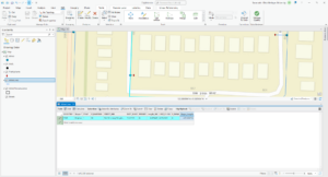
  • Snapping allows you to connect features, without impossibly precise sketching

Questions and Screenshots:

  • (Configure snapping options 8) The selected line has 4 vertices
  • (Split polygons 12) The Shape_Area value decreased

Getting to Know ArcGIS Chapter 5

Notes:

  • Tasks can be documented series of instructions that incorporate or call forth certain tools and commands
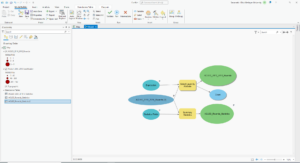
  • ModelBuilder is a geoprocessing environment that allows you to easily link one tool to another and run one set of operation after another
  • In the “Tasks” pane you can follow or define a workflow

Questions and Screenshots:

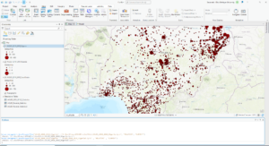
  • (Set up a project 4) The conflict events recorded in the dataset are battle (government regains territory), battle (no change of territory), battle (non-state actor overtakes territory), headquarters or base established, non-violent transfer of territory, remote violence, riots/protests, strategic development, and violence against civilians
  • (Author a task 12) 14,211 fatalities resulted from violent conflicts against South Sudanese civilians between 2010 and 2018 
  • (Fill out the tool parameters 5) 71 fatalities resulted from violent conflicts against Rwandan civilians between 2010 and 2018 
  • (Convert a model to a geoprocessing tool) 41 riots/protests occurred in Rwanda between 2010 and 2018 and 12 fatalities resulted from these events
  • (Use a custom script tool 1) The geoprocessing tools of “Select Layer by Attribute” and “Summary Statistics” are combined in the script
  • (Use a custom script tool 6) 26,323 fatalities resulted from violent conflicts against Nigerian civilians between 2010 and 2018 


Week 3 – Savannah Domenech

Mitchell Chapter 5:

Key concepts and definitions:

Boundary: a polygon that is placed on top of features and is used to select features within in order to list or summarize features or in order to combine the boundary and features to create summary data. Boundaries can be shaded areas that go in front or behind the outer area (this emphasizes the area itself) or they can be thick lines (this emphasizes the inner area).

Drawing areas and features: a method that allows you to visually find out whether features are inside or outside the boundary. This method is for working with one area.

Selecting the features inside the area: a method that provides a list or summary of features inside the boundary. This method is for working with one area.

Overlaying the areas and features: a method that determines which features are inside which boundaries and also summarizes features by area. This method is for working with several areas or single areas. Using the raster model is more efficient than using the vector model.

Count: the total number of features inside an area or boundary.

Frequency: the number of features with a certain value inside an area or boundary displayed as a table or chart.

Slivers: very small areas where areas are slightly offset from overlaying. Slivers should be merged into adjacent larger areas according to minimum mapping unit and data accuracy guidelines.

Minimum mapping unit: the smallest area input in a dataset.

Notes and Questions:

  • Finding what’s inside a single area lets you monitor activity or summarize information about the area and finding what’s inside numerous areas lets you compare the areas
  • You want to include features that are partially within the boundary if you are gathering a list or count of features
  • When looking to determine the amount of something within a boundary, you would only include the portion inside the area
  • Am I correct in understanding that overlaying the areas and features is selecting the features inside the area just with an additional step and that selecting the features inside the area is drawing areas and features just with an additional step?


Mitchell Chapter 6:

Key concepts and definitions:

Traveling range: determines what’s within a set distance of a feature. Distance, time, or cost can be used.

Travel costs: often termed the impedance value. Time, distance, and money are very common.

Planar method: used for calculating distance on a flat earth and in a relatively small area.

Geodesic method: used for calculating distance taking into account the curvature of the earth and in a relatively large region.

Inclusive rings: useful for determining how the total amount of something increases as distance increases.

Distinct bands: useful for comparing different distances to other characteristics.

Spider diagram: formed when GIS draws a line between each location and its nearest source. They are useful for comparing patterns between two or more source points.

Junctions: points where edges meet.

Turns: used to determine the cost to travel through a junction.

Edges: street segments or lines.

Turntable: a data table that contains the junctions which you want to assign a cost to.

General boundary: it connects the farthest reaches of the selected segments (forms a blob).

Compact boundary: it outlines the selected segments.

Mask layer: used for blocking the assignment of cost values to cells. You would assign the cells a very high value or no value at all to do this.

Notes and Questions:

  • Area of influence is typically measured using straight-line distance (putting a boundary of a certain radius, depending on the distance specified, around the chosen feature)
  • Travel movement is measured over a geometric network (for example roads). Travel costs can also be applied to this
  • Cost over a surface is used for overland travel and is useful for showing rate of change. It uses the raster model
  • When finding features near several sources you need to create separate straight-line buffers otherwise you won’t know which source (or sources) the feature is near
  • You should specify the maximum distance when finding what’s nearby
  • Distance ranges are created using graduated colors
  • If you need to be specific when calculating travel time (cost) include turns and stops
  • The source should be a different, distinguishable symbol than other features
  • To create a cost layer based on a single factor reclassify an existing layer for the attribute you want, and to create a cost layer based on numerous factors combine all the layers together after reclassifying each input layer
  • I understand the theory of how to find what’s nearby but I don’t know the technical steps to take


Mitchell Chapter 7:

Key concepts and definitions:

Time patterns (trend, before and after, and cycle): a trend map represents change between two or more times, a before and after map represents change preceding and following an event, and a cycle map represents change over a recurring period of time.

Tracking map: shows the position of a feature or features at several times. This is useful for showing incremental movement and geographic phenomena.

Trendline chart: shows a relative value as well as that value’s growth over time.

Notes:

  • You can map change by creating numerous maps showing the condition of features at each time or by calculating and mapping the difference in value for each feature
  • When mapping trends you need to determine the time interval
  • When mapping cycles you can map either snapshot or summarized data
  • When mapping before and after you want to use snapshots as close as possible to the event
  • When mapping discrete events you need to use summarized data and when mapping continuous data you can map summarized or snapshot data
  • Time series maps are good for showing changes in boundaries, values, or surfaces. You create one map for each time; however, you shouldn’t have more than six maps
  • A tracking map is good for showing movement in boundaries, lines, and discrete features
  • When mapping change in magnitude use the same classification scheme for all the maps
  • Quantile and equal interval schemes are useful for comparing values over time
  • You can generalize categories if historical categories vary from existing categories
  • To show movement in a trend map use different colors for each time period, to show movement in a before and after map use one color to represent the before and one color to represent the after, and to show movement in a cycle map use different colors for each time period
  • To emphasize the “from” in “from → to” change, map those categories in shades of the same color, and vice versa if you want to emphasize the “to”

Savannah Domenech Week 2

Mitchell Chapter 1:

Key concept and definitions:

GIS analysis: The steps that are taken to find geographic patterns in a dataset and to find relationships between features.

Types of features (discrete, continuous, summarized by area): Discrete features can be pinpointed. Continuous features blanket the entire area and usually start off as a series of points which are then interpolated. Features summarized by area have a data value applied to the entire area which represents the sum or density of certain individual features within that area.

Interpolation: When GIS assigns values to areas in between points to create continuous phenomena.

Vector model: Every feature is a point, line, or polygon and a row of data in the attribute table. It uses coordinate data. Discrete features, continuous features, and features summarized by area are represented using the vector model.

Raster model: Every feature is a matrix of cells in continuous space; the size of the cells can be adjusted (too large and data is lost, too small and it takes a long time to process and doesn’t add additional precision to the map). Continuous features and numeric values are represented using the raster model. 

Map projections: They allow data to be viewed on a globe which is transformed to be a flat surface. Different map projections distort area, distance, and direction differently. 

Notes:

  • Making maps is in effect analysis. Models (with many layers) also are analyses
  • The steps to analysis are: frame the question (be specific!), understand your data (figure out what you have and might need so you can get the information you want), choose a method (there are faster, less precise ways and slower, more precise ways), process the data in GIS, and look at the results (which can be a map, a table, or a chart)
  • The types of attribute values include categories, ranks, counts, amount, and ratios
  • A purpose of GIS analysis is to find why things are where they are and how things are related
  • I learned my first little bit about raster data and the raster model


Mitchell Chapter 2:

Key concept and definitions:

Subset: Only using certain attributes of a larger data set (for example, theft is a subset of crime).

Distributions: Features that are clustered are likely to be near other features, features that are uniform are less likely to be near other features, and features that are random have the same likelihood to be at any given location.

Notes:

  • Many patterns can be determined just by mapping a phenomena
  • It is important to consider your audience, medium, and purpose when mapping
  • You can map more specifically or generally depending on your purpose; the goal is to make patterns easy to see
  • Single codes can indicate both major type and subtype (for example, codes 500 to 599 are burglary and each number in between is a specific type of burglary)
  • You shouldn’t display more than seven categories on a single map
  • A general rule of thumb is to use less categories when zoomed out on an area, however when you are zoomed in on an area you can use more categories
  • There are trade-offs in mapping; using fewer categories can make a map and patterns easier for the audience to understand but information is lost by reducing or condensing numerous categories into fewer categories
  • Three methods of grouping categories are: assigning a general code to each more detailed record in the database, creating a linked table that matches detailed codes to general codes, and assigning the same symbology to certain detailed records to visually create a more general map. The first two involve using the Attribute Table and the last one is more artificial and involves using classification
  • It’s harder to distinguish shapes than colors
  • Since it can be different to distinguish narrow line colors, consider using different thicknesses or patterns (dotted, dashed, etc.) for lines
  • Mapping reference features can be important as it gives people a visual bearing at what they are looking at. This should be done using non-dominant colors


Mitchell Chapter 3:

Key concept and definitions:

Counts and Amounts: Counts are the number of features on a map and amounts are the values attributed to each feature on a map. Both show total numbers and can be used with discrete or continuous phenomena.

Ratios: It is formed by dividing one quantity by another. They are useful when summarizing by area and will typically be averages, proportions, or densities.

Ranks: It is a relative ordering system rather than a measured one.

Classes: It is grouping values into groups so values that fall into a certain break are a part of one group and values that fall into a different break are part of another group . Counts, amounts, and ratios are usually grouped into classes.

Classification schemes (natural breaks, quantile, equal interval, and standard deviation): Natural breaks emphasize differences in values. Quantile schemes put an equal amount of values into each class. Equal interval schemes form classes with equal ranges. Standard deviation schemes form classes based on how values vary from the mean. 

Notes:

  • Discrete phenomena can be represented using graduated symbols (points and lines), graduated colors (areas), or sometimes 3D perspectives (all)
  • Continuous phenomena (areas) can be represented using graduated colors, contours, or 3D perspectives
  • Features summarized by area can be represented using shading
  • Features with similar values should be in the same class and there should be as great as a difference possible between classes
  • Most people can determine up to seven colors on a map
  • Reds and oranges attract the most attention and blues and greens the least
  • Some ways of dealing with outliers include: putting each outlier in its own class, grouping outliers into one class, grouping outliers with the next closest class, or denoting them using a special symbol
  • Circles are the most distinguishable graduated symbol
  • You can use charts to show more information on a map, but don’t show more than five categories on a chart and don’t map more than thirty features
  • Contour lines are used to show the rate of change for a spatially continuous phenomenon (like pressure lines)
  • 3D perspectives have three parameters: viewer’s location, vertical exaggeration, and location of light source


Mitchell Chapter 4:

Key concept and definitions:

Cell size: It determines how fine (smaller cells) or coarse (larger cells) patterns will be. Cells are square and in general there should be between 10 and 100 cells per density unit.

Search radius: The larger the radius the more generalized the patterns. 

Calculation method (simple and weighted): The simple method only counts features within the search radius so that each cell has the potential to have a ring around it. The weighted method emphasizes features more near the center of a cell and results in a smoother, more generalized surface. 

Units: If areal units are different from cell units the values are extrapolated.

Centroids: Center points.

Notes:

  • Density maps show you where the highest concentration of features are
  • Density can be mapped using a dot map, by calculating the density for each area, or by using density surfaces
  • Dots on density dot maps are distributed randomly throughout the area they correlate to
  • Dot maps are good for giving a quick sense of a specific area’s density
  • On dot maps, dots are often displayed based on smaller areas but the boundaries of larger areas are typically visually shown
  • Density area maps should use a range of color values with one or two hues
  • Density surfaces are usually created as a raster layer, are good at showing where points and lines are concentrated, and can be created using graduated colors (using shades of a single color) or contours
  • Density surfaces are created by defining a search radius around each cell center and then GIS calculates how many features or values that cell radius contains and divides it by area or another value
  • Just because there is a high density portrayed on the map does not mean there are actually any features in that cell; this is the result of a search radius that is picking up other features
  • Density surface maps were the most confusing thing for me in these four chapters

Savannah Domenech Week 1

  1. A basic introduction to you with a glossy 8.5×11 photograph

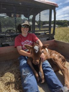
I am Savannah Domenech and I’m from the Greater Rochester Area in New York (in particular Webster, NY). I am an Environmental Studies and Geography major. This is my third semester of having Dr. Krygier as a professor in a row. A fun fact about me is I wanted to be a firefighter growing up (and still do have some interest in doing it as a volunteer perhaps one day). I have other fun facts too, like I carried two brand new baby calves this summer; they were heavier than I thought! Below is Caramel, born in the early afternoon of June 28th. 

2. Read Schuurman ch. 1 (PDF) & include a few comments, thoughts, etc.

  • GIS sure has a lot of uses from Starbucks store planting to epidemiological identification. One use that stood out to me (as I was a farming intern this summer) was using GIS to determine why a certain area of a crop field is not doing well. I also did not realize GIS is used to plan out garbage truck routes
  • Overall, the chapter suggests that the two main uses of GIS are making maps and analyzing data
  • The article raises the good point that GIS is overshadowing other valid and useful data collection and visualizing methods (like qualitative human geography methods and radar). Honestly, when I thought about radar I thought about how radar could be translated into GIS, not that radar can be its own separate entity
  • I also learned that GIS can stand for Geographical Information Science as well as Geographical Information Systems. Systems is more of the final product while Science is the behind the scenes work and algorithms that deeply influences the final product. I really liked what the chapter said: that Systems is “‘where’ spatial entities are or might be” and that Science is “‘how’ we encode spatial entities… and the repercussions of different methods of analysis on answers to geographical questions.” But I agree with the chapter when it says there is a fuzzy boundary between the two
  • Before reading this chapter I thought that GIS was primarily for interactive mapping, I did not really consider its other uses
  • Something important to keep in mind is that layer overlay is the basis for spatial analysis. In addition, the difference between mapping and spatial analysis is that mapping propositions geographical data in a visual form and does not create more information while spatial analysis extracts information from spatial data. In particular, computers are excellent in solving spatial questions and performing spatial analysis. With this in mind, one thing I am curious about is the delineation between spatial and geographical data
  • I did not realize GIS’ origins were so debated and complex
  • I think the point the chapter makes about the necessity of understanding the question (and what data is appropriate to that question) you are proposing is essential. If this is not done right the map’s purpose can easily become muddled or the data could be not applicable to the question
  • The chapter also rehashed an important concept from GEOG 112: that images (such as maps) have power and that maps allow the data to be visualized in a much better sense than just looking at a huge chart of data (like my South Carolina maps I made in GEOG 112). Furthermore, the chapter points out that while maps help us to see patterns, spatial analysis allows us to be more precise about those patterns
  • Also, reemphasized from GEOG 112 is that classification scheme breaks and polygon areas can deeply affect the visual meaning of a map but often most people do not consider why they were chosen and how they correspond to the creator’s interpretation of the data. We need to think about the underlying assumptions that we contribute to our maps, such as symbology, but also consider the underlying assumptions written into the code of GIS
  • I also learned through this chapter that GIS can be used to predict future events


3. Use Google and Google Scholar to look into a few GIS application areas: search for “GIS Application” and different keywords, based on your personal interest: wolf telemetry, LGBT, carnivorous plants, hate groups, crime, sewers, crowdsourcing, etc.). Include, in the blog posting, information on two applications with at least one map or image and a source or two. 

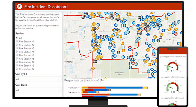
Fire Operations | Incident Command Software & Reporting Using GIS

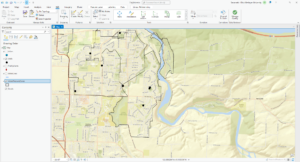
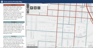
  • Finally, I wanted to look into GIS applications for the City of Delaware. One GIS application I found was the City of Delaware’s Snow Priority Map which is important because now students can know why (and also which) roads are and are not cleared quickly.Â