Author: sdroberts

 

Chapter IV

 

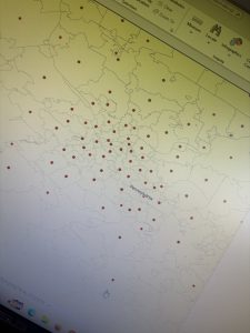
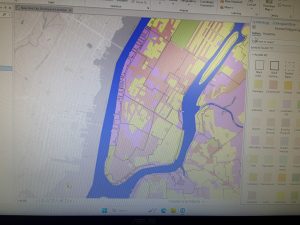
Chapter four is entirely focused on density based mapping. At first I believed this chapter was going to feel like a tedious slog, given that density based maps do away with precise location in favor of a more relative form (such as population per square mile). Effectively mapping density is a trade off from point based data to quantitative data which I believe to be somewhat redundant given that point based data typically tend to show density anyways.

However, upon reading the chapter I do believe that density mapping has its uses, especially when cross examined with more point driven data. An example the textbook gave for this was comparing sights of crimes with regional information on average income in the areas or reported gang activity. 

The GIS software does plenty of work as far as plotting and interpreting the density based data goes, including totalling the number of values within a designated area and dividing it equally across the size of the area in question as well as both general averages of the data and weighted averages.

Much of the general advice from the previous chapters apply here as well. One which I feel is a little bit redundant at this point is the specification on the classes of value a density map should have to be easily readable. This is something that was discussed in the previous chapters relative to the different classes of point based data. (More point classes makes the map harder to read, applies the same to value classes in density mapping)

 

Chapter V

 

Finally I am getting to exciting things! Mapping within a certain radius and interpreting data within that is the kind of geographical analysis I took this class to learn about.

The chapter designated several types of area based maps: Single areas (Within a single area, it is in the name) Buffers (an area surrounding a certain feature or features) and boundaries. (the boring one)

There is also a distinction to be made between the maps I just discussed and mapping multiple areas, such as contiguous areas which typically are located right next to each other, and Disjunct areas which have “buffer land”.

Then the chapter discusses discrete and continuous features. We have been over this.

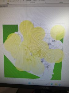
The GIS software is capable of several methods of analyzing limited maps. The book has the example of a flood map and shows the GIS being able to find specific designated areas that may fall within or without the flood path, as well as being able to count and/or list the designated areas within the flood path. There is even the ability to create distinctions between the areas and categorize them by value or type based on whether they fall within the designated focus area or create visual data representations based on the data within the areas.

 

Chapter VI

 

I feel the subject matter of this chapter overlaps considerably with the previous chapter. Once again, this is based nearly entirely on mapping within a certain area. The primary difference being the discussions on how the GIS software can calculate the distance (or cost) and possible travel routes. 

Of course, nothing fun is ever easy and frankly a wrench was thrown into my ideas on applying this when the book discussed the differences between miles based on a certain geographical projection (effectively assuming the earth is flat) and based on the curvature of the earth. I hope the difference between these values will not be too big of an issue given the rather limited area I intend to map, but I know for a fact if I were mapping a larger scale project that this would potentially derail my analysis completely. 

The book describes the differences between different methods of mapping using proximity as the primary considerations as well as discussing the measure these methods record and which situations these can be applied in.

I actually really enjoyed reading about the cost over surface method. I am currently reading about the construction of the first trans-continental railroad which used a great deal of cost over surface mapping when surveying the land and even using that to modify the land to be better suited for rail transportation. (The TV show Hell on Wheels famously depicts a “cut crew” who would dig up large amounts of earth to construct a level railbed.)

This leads into the next thing I thought was interesting: Networks. Using lines that can represent road, railroads, or airways the GIS can automatically calculate the distance or cost by only following the network to the intended destination. I feel like that is one of those things that is so obvious to the common man that it effectively vanishes from our consciousness.

Chapter 1:

 

The first chapter I found to be rather uneventful. Merely being a basic rundown of the different features of GIS software and general GIS terminology students should be aware of. I personally found the way the textbook categorized the terminology to be somewhat confusing at best and forcing me to re-read the same pages several times at worst. The way I understood the textbook’s definitions of different GIS uses was that they are divided into two categories: Discrete locations which represent individual points, lines and areas which are easily separable and can be viewed in a vacuum, and continuous phenomena which describe much more intertwined data that relies on the geography surrounding it. (Such as ground elevation or surface temperature.)

Other features discussed in this chapter include how GIS software can present geographic attributes relative to the different points/regions/whatever put on the map. Although this is at first glance a very useful feature, I have general concerns as to the level of data these charts can present. The textbook categorizes the types by value but I know for a fact I would want to put more “general” notes on the maps I create (yeah, I am that guy) and my experience using different specialty software to create generalized notations have varied widely and if I do pursue the geographic analysis of the Whitechapel murders in this class I know for a fact I would be adding notes pretty much everywhere and the examples of the data tables in the textbook shows very little capacity for my notes and whatnot.

 

Chapter 2:

 

The beginning of the second chapter talks about the practical applications of geography and cartography. I think given how much people still rely on maps, even in the digital age, the points given are rather obvious. Therefore most of my notes will be on the reminder of the chapter. 

This is a small thing but I love the emphasis on geographic coordinates the textbook stresses. Reading and writing coordinates is a very useful but sadly dying skill and I’m glad that it will play an important role in this class and that we will be learning the exact coordinates of the points of data plotted on our maps.

I’m also very excited to use the subsets on my maps. I personally love organizing things and reading this chapter I was absolutely blown away by the amount of options the textbook referenced how the various data points could be organized by and how you have the option to only view data points under a certain classification in your analysis or even displaying the features by type. (It’s probably dangerous for me to have this power.) The chapter also discussed the visual science of analyzing a map, such as organizing data points into broad categories to avoid confusion and labeling the data points in different colors, but no more than seven colors. 

 

Chapter 3:

 

This chapter summed up the critical thinking aspect of mapmaking quite well and stressed the idea of finding relationships in the data across geographic and numerical lines. (or as the textbook referred to it, “mapping the most and least”) This is also where the textbook begins discussing the mathematical values within geography. Many instances reminded me of my high school statistics class.

Luckily for me, most GIS softwares (at least according to the reading) can aid in calculating the stats and preparing them for analysis. 

However, the classification schemes look rather difficult to deal with. Midway through the chapter, there are several tables displaying the advantages and disadvantages of using each one. (Nothing worth doing is easy I guess) Given the rather point focused data I will be experimenting with in this class, I wonder if any of these classification schemes are applicable, or even worth doing in the first place since many of the examples in the textbook using them represented maps analyzing continuous phenomena and/or maps with different data values per region that are being analyzed. 

Moving towards the realm of the types of digital maps presented by the textbook, they show a similar story to the classification schemes in regards to practicality in terms of the situation at hand. I will admit I found the 3D maps to be a somewhat corny feature at best and an outright terrible way to display data at worst. Though it is undoubtedly the most versatile of the map types discussed in the textbook in terms of what can be marked, it still (in my opinion) shows very little point by point data, can be very confusing to read, and honestly just looks tacky.

I know for a fact that the Graduated Symbol map would be my go to on the more independent projects for they look ideal for the kind of geographical criminal profiling I want to do in this course.

Yes, I did take the quiz.

I go by Gustav but my boring name is Samuel. I am an english major who is taking this class as an upper level Gen Ed.

I found the chapter to be very interesting.  When I was given the introduction to this class I had ben informed of the multi-disciplinary applications this knowledge could have but reading the chapter really put things into perspective for me, as the chapter seemingly had a way to trace nearly every sector of out lives back to GIS applications. I especially found the passages regarding the applications for precision farming and for utility companies to be particularly interesting given that I feel those are sectors of life that most people don’t give much of a second glance at in day to day life and it is very enlightening to see just how much work goes into these fields using GIS alone all for the common man to simply ignore them on the basis of “out of sight, out of mind”.

I think my biggest takeaway fro the chapter was the knowledge on the subject of GIS itself. My first impressions as someone who had never seen that acronym before was that was the name of a commonly used computer program sed to conduct geographical analysis in a similar way to how business students are taught to use Microsoft Excel or how Engineering students are taught with Autodesk Inventor. Upon reading more (and coming across the interesting history of GIS dating back to the 19th century which I found to be absolutely fascinating) I found out that my initial assumption was quite wrong and that GIS is much more of a scientific field in itself given the vast ways geographical data could be gathered and interpreted.

 

The main application I am curious about is Geographical Criminal Profiling. I have a minor interest in criminology (though I have received no formal education on the matter) and GCP is very commonly used in many criminal investigations.

Source: https://atlas.co/gis-use-cases/geographic-profiling/

Something I think would be interesting to do in this class is using the GIS software I could create a geographical profile of the infamous Jack the Ripper murders in the autumn of 1888. I find most maps on the subject (below) tend to be rather unenlightening and not particularly interesting for nerds like me as they tend to include many non-canonical events in their analysis  (The map I have included in this post from Wikimedia commons is one of the worst offenders in my opinion) and I personally would like to see one based much more in the facts rather then the insane amount of theories.