Tax District
This data set contains tax districts in Delaware, OH. It is from the Auditor’s Real Estate Office. It is updated as needed.
Parcel
This data set contains the cadastral parcel lines in Delaware, OH. It is maintained by the Auditor’s GIS Office. Records are in the County Recorder’s Office, and individual records are in the CAMA system. It is updated daily.
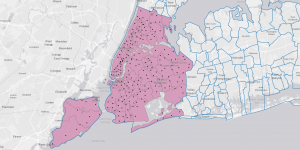
Address Point
This data set is a representation of certified addresses in Delaware, OH. It is maintained by the Auditor’s GIS Office. The Address_Points layer is for appraisal mapping, 911, accident reporting, geocoding, and disaster management. It is updated daily.
Recorded Document
This data set consists of points that represent documents in the Recorder’s Plat Books, Cabinet/Sides, and Instruments Records. These documents include vacations, subdivisions, centerline surveys, annexations, and other documents. It is updated weekly.
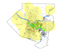
Zip Code
This data set contains zip codes in Delaware, OH, and was created in 2005. Some places were either tax-exempt or had no zip codes, so they were manually populated. The layer was created from data from the Census Bureau, USPS, and tax mailing addresses from the treasurer. It is updated as needed.
School District
This data set contains the school districts in Delaware, OH. It is created from the County Auditor’s records. It is updated as needed.
Map Sheet
This data set contains the map sheets in Delaware, OH.
PLSS
This data set contains all the Public Land Survey System data in the US Military and Virginia Military Survey Districts of Delaware, OH. It is updated as needed.
MSAG
MSAG stands for Master Street Address Guide. This data set contains the 28 political jurisdictions in Delaware, OH. It was created for locating boundaries of cities, villages, and townships in the county. It is updated as needed.
Municipality
This data set contains the municipalities of Delaware, OH.
Farm Lot
This data set contains the farmlots in the US Military and Virginia Military Survey Districts of Delaware, OH. It is used to identify the farmlots and their boundaries. It is updated as needed.
Township
This data set contains the geographic boundaries of the 19 townships in Delaware, OH.
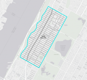
Street Centerline
This data set depicts center pavement on all roads in Delaware, OH. It was collected by field observation. It is used for appraisal mapping, 911, accident reporting, geocoding, disaster management, and roadway inventory. It is updated daily and the 3-D fields are updated annually.
Annexation
This data set contains annexations and conforming boundaries in Delaware, OH from 1853 to present day. It is updated as needed.
Condo
This data set contains the condominium polygons in Delaware, OH. The data is from the County Recorder’s Office.
Subdivision
This data set contains the subdivisions and condos in Delaware, OH. The data is from the County Recorder’s Office. It is updated daily.
Survey
This data set contains a shapefile of points that represent surveys of land in Delaware, OH. The data is from the Recorder’s office and the Map Department. Old Survey Volumes are not included. Some surveys are still being scanned. It is updated daily.
Dedicated ROW
This data set consists of right-of-way roads in Delaware, OH. It is updated as needed based on parcel data. All changes are recorded in the County Recorder’s Office and updated daily.
Building Outline 2024
This data set contains the outlines of all buildings in Delaware County. It was last updated in 2024 and is updated as needed.
Building Outline 2023
This data set contains the outlines of all buildings in Delaware County. It was last updated in 2023 and is updated as needed.
Railroads
This data set contains the railroad lines in Delaware, OH. It was digitized by the County Auditor’s GIS Office from ortho photography corrected from 1997 to 2002 and 2006.
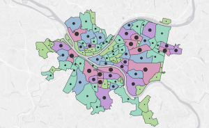
Precincts
This data set consists of voting precincts in Delaware, OH. It is maintained by the County Auditor’s GIS Office. It is updated as needed.
Delaware County E911 Data
This data set contains an accurate representation of certified addresses in Delaware, OH. It is used for appraisal mapping, 911, accident reporting, geocoding, and disaster management. It is updated daily.
Building Outline 2021
This data set contains the outlines of all buildings in Delaware, OH. It was last updated in 2021 and is updated as needed.
Hydrology
This data set consists of major waterways in Delaware, OH. It was enhanced with LIDAR data in 2018. It is updated as needed.
GPS
This data set has GPS monuments established in 1991 and 1997 in Delaware, OH. The coordinates are in Universal Transverse Mercator Northing and Easting. It is updated as needed.
Delaware County Contours
This data set contains two foot contours from 2018.
Original Township
This data set contains the original boundaries of townships before tax district changes in Delaware, OH.