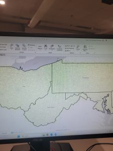
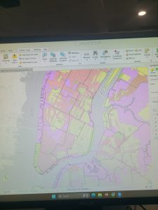
This week I basically just downloaded all the data needed for my final project. I explored the Delaware County, Ohio GIS Data Hub and looked through the datasets available in the “All Files” section. I downloaded Parcel, Street Centerline, Hydrology, and Township Boundary shapefiles. I also extracted them and exported them to ArcGIS. In terms of what they each do: Parcel outlines property boundaries across the county, Street Centerline layer displays the county’s road system, and Hydrology layer identifies streams and other water features. For my final project I also had to download the subdivision shapefile because I decided to do”Mapping Change” as well as “Making New Shape Files from Existing Shape Files”.
Author: jlspurling
Spurling Week 6
Chapter 7-
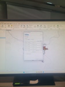
I found chapter 7 tutorials relatively easier. In this chapter, I worked on split features, zooming and formatting different buildings on a map. For example, I opened the Baker Porter bookmark and was able to split the polygon successfully. Overall, I really enjoyed this chapter and found enjoyment in editing buildings on the map. 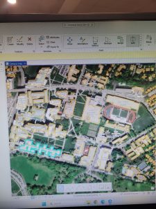
Chapter 8
For some reason I could not how to navigate this chapter at all. I was unsuccessful in finding the create locator tool which was a major part of the tutorial. However, overall this chapter was about navigating different regions and geocode data by zip code.
Chapter 9
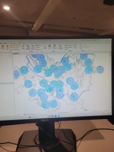
This chapter redeemed the last chapter. This chapter helped me learn about the pairwise buffer tool. I was able to successfully use it and use it for the whole chapter/tutorial. I also learned about the proximity analysis.
Spurling Week 5
Chapter 4
I found this chapter a little hard to navigate solely because of the “adding clauses” section of the tutorial. However, other than that, I was able to do the rest successfully. I now feel more comfortable working with GIS in general, and I feel capable finding and completing basic tasks.
Chapter 5
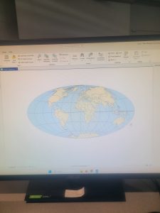
After Chapter Four’s difficulties, this chapter and tutorials made me feel a lot better. This chapter was all about spatial data. The Hammer-Aitoff projection is also pretty cool to be able to create. The only discrepancy I had was specifying the display units for the map, however, other than that, it was fine.
Chapter 6
This chapter is about geoprocessing. This chapter was also a little harder than I anticipated as well. The pairwise dissolve tool was okay at first, but the more I used it the harder I found it to navigate. Overall, I feel good about this week’s chapters and feel more confident in my GIS abilities
Spurling Week 4
Chapter 1
I learned how to start making a basic map using GIS software. I practiced adding layers to a map and understanding how different layers represent different types of information, like locations, boundaries, and features. I also learned how to navigate the map, zoom in and out, and adjust how the data is displayed. I found this tutorial very easy, and starting out with Allegheny, Pennsylvania, made me feel very confident.
Chapter 2
I learned how to improve a map by using colors and symbology to represent different parts of a city. I worked on changing the appearance of map layers so that different areas were easier to see and understand. This helped show how maps can communicate information visually, not just display locations. The most challenging part for me was finding and selecting the exact colors needed for each section.
Chapter 3
I worked on creating two different maps, which made this chapter the most challenging for me. I had to repeat many of the same steps for the second map, and I often got lost trying to remember what to do next. This chapter helped me practice staying organized and understanding the full mapping process from start to finish. I also struggled with creating and formatting the title rectangles, but after some trial and error I was able to figure it out.
Spurling Week 3
Chapter 4-
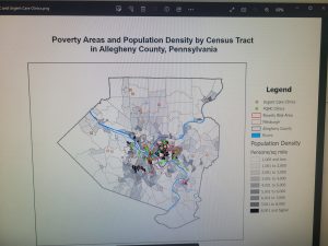
Chapter 4 highlights why density mapping is such an important GIS tool. Simply plotting locations shows where things exist, but density mapping shows where they’re actually concentrated and where they thin out. Looking at values per unit area makes spatial patterns much easier to notice and compare across a region.
One thing the chapter makes clear is that there isn’t just one way to map density. In some cases, using predefined boundaries like counties or census tracts works best. This approach calculates density within each area and usually shows up as shaded polygons. It’s helpful for comparing regions, but it can also be limiting since internal variation gets hidden by those boundaries.
Another option is density surface mapping, which creates a continuous surface instead of sticking to fixed borders. Density values are calculated for each raster cell based on nearby features within a chosen distance. These maps are better at showing gradual changes and identifying hotspots, which makes them feel more realistic. At the same time, they take more processing power and require more careful decisions.
Chapter 5-
Chapter 5 is all about answering the question of what is actually inside something else. Instead of just mapping layers and looking at them separately, this chapter explains how GIS can be used to figure out which features fall within certain boundaries. It feels like one of the most useful parts of GIS because it connects maps directly to real questions.
A big idea in this chapter is spatial overlay. This is when different data layers are stacked on top of each other to see how they interact. Depending on the tool you use, such as intersect or union, you end up with different results and keep different pieces of information.
The chapter also talks a lot about containment, which is figuring out whether points, lines, or polygons fall inside another feature. It sounds simple, but it becomes really powerful when applied to real situations. Things like counting how many schools are within a certain area or identifying neighborhoods located in an environmental risk zone feel very doable using GIS.
Something that stood out to me is how careful you have to be with your data. If layers do not line up correctly or boundaries are inaccurate, the results can easily be off. The chapter makes it clear that GIS is not automatic or perfect and that users still need to think critically. Overall, Chapter 5 makes GIS feel more relevant and useful.
Chapter 6-
Chapter 6 focuses on figuring out what is nearby and why distance matters in GIS. Instead of just asking what is inside certain boundaries, this chapter looks at how close things are to each other and how that closeness can affect analysis. This feels useful because so many questions depend on distance, like access to services or exposure to certain conditions.
The chapter talks a lot about proximity analysis, which is used to measure distance between features. One common method is creating buffers around points, lines, or areas to see what falls within a certain distance. Buffers make it easier to answer questions like which schools are within a mile of a park or which homes are close to a major road. I liked how this made distance feel more concrete instead of abstract.
Another important idea in this chapter is choosing how distance is measured. Distance can be straight line or based on actual travel paths like roads or sidewalks. The chapter points out that this choice can change results a lot, which made me realize how important it is to think about what “nearby” really means in each situation.
Spurling Week 2
Chapter 1
Chapter 1 introduces GIS as a tool for identifying and making locations and patterns. Overall, this chapter felt pretty uneventful because it mostly reviewed ideas that seem straightforward, such as using maps to understand where things are and why they are there. Mitchell also focuses on the idea that GIS is not just about making maps, but about using spatial data to answer questions and support decision making. Some vocab words were vector and raster data, which are two basic ways GIS represents spatial information. Vector data uses points and lines to show exact locations. Raster data represents space as a grid of cells, with each cell holding a value, and is used for things like elevation or temp. While vector data focuses on precision and defined features, raster data is better for showing continuous patterns across an area. While this distinction is important, much of the chapter felt like setup rather than new information. Even though the chapter was not very exciting, it did help establish the foundation for the rest of the book. It clearly explains why spatial thinking matters and how GIS can be used to identify patterns and relationships that might not be obvious in other data.
Chapter 2
In chapter 2, the focus shifts to how identifying locations and features helps explain the patterns you start to notice on a map. A lot of this chapter is about making choices, like deciding what information is actually worth mapping and how that choice affects what the map shows. GIS can take things like addresses or latitude and longitude points and turn them into mapped features, which helps give structure to otherwise scattered information.
I found it interesting how much emphasis was placed on categorizing features, since mapping by category can change how a place is understood. At the same time, the chapter points out that too many categories can make a map hard to read, which is why it suggests keeping the number fairly limited. ArcGIS basemaps also came up as a way to give context to your data. When looking at geographic patterns, features can appear clustered, evenly spaced, or random, and mapping the highest and lowest values adds another layer of meaning to the patterns you see.
Chapter 3
In Chapter 3, it really builds on the earlier chapters by showing how much interpretation and decision goes into making a map. The chapter made it clear that maps are not neutral, since every choice really illustrates something to the observer or maker. The purpose of the map shapes how information is presented, whether you are trying to simply observe relationships or highlight a specific pattern. This chapter also discusses different types of quantities, such as counts, ratios, and ranks, and explains that each needs to be represented in a different way than the other.
I liked that this chapter emphasized having a clear question before choosing an analysis method. It showed that GIS is a step by step process rather than just experimenting with tools. This chapter connected the ideas from earlier chapters to real applications and made GIS feel more concrete and useful. Overall, this chapter was the most helpful in terms of understanding how GIS can be applied.
Spurling Week 1

Introduction: My name is Jessie Spurling, and I am a senior majoring in Biology and Psychology. I’m from Lancaster, Ohio (Hocking Hills area). My on-campus activities include being on the softball team, a tour guide, and a member of the Delta Zeta sorority. After college, I intend to pursue a career in conservation/ecology or environmental education, and I feel that GIS will significantly help me with those future endeavors.
Schurmann Chapter 1: In the first chapter of GIS: A Short Introduction, Schuurman explains what Geographic Information Systems (GIS) are and why they are important. She starts by defining GIS as a way to collect and analyze data that is connected to location. What stood out to me most is that she makes it clear early on that GIS is not neutral. Even though maps and data often look objective, they are created by people, which means human choices and biases are always involved (boo).
Schuurman also explains how GIS works by combining maps, databases, and computer technology. She talks about layering data, such as putting population information on top of environmental or political data, to better understand patterns and relationships. This helped me understand why GIS is such a powerful tool and why it is used in so many areas like city planning, environmental studies, and public health.
Another important point in this chapter is how much influence GIS can have. Schuurman explains that because GIS outputs look scientific and authoritative, they are often trusted when making decisions or policies. However, she warns that if the data going into GIS is incomplete or flawed, the results can still look convincing even if they are inaccurate. This made me think more critically about how much we trust maps and data without questioning where they come from.
GIS Applications: The first GIS application I looked at was Assessment of habitat suitability and connectivity across the potential distribution landscape of the sambar (Rusa unicolor) in Southwest China. This application uses GIS to map where sambar deer are most likely to live and how different habitat areas are connected. I focused on the habitat suitability map, which shows areas ranked from low to high suitability. Darker shades on the map represent areas that are more suitable for the sambar.
I noticed that the most suitable habitats were clustered in mountainous and forested regions of Southwest China, while areas with lower suitability appeared in more developed or fragmented landscapes. Some of the high-suitability areas were separated by large regions of low suitability, suggesting that the habitat is not well connected.
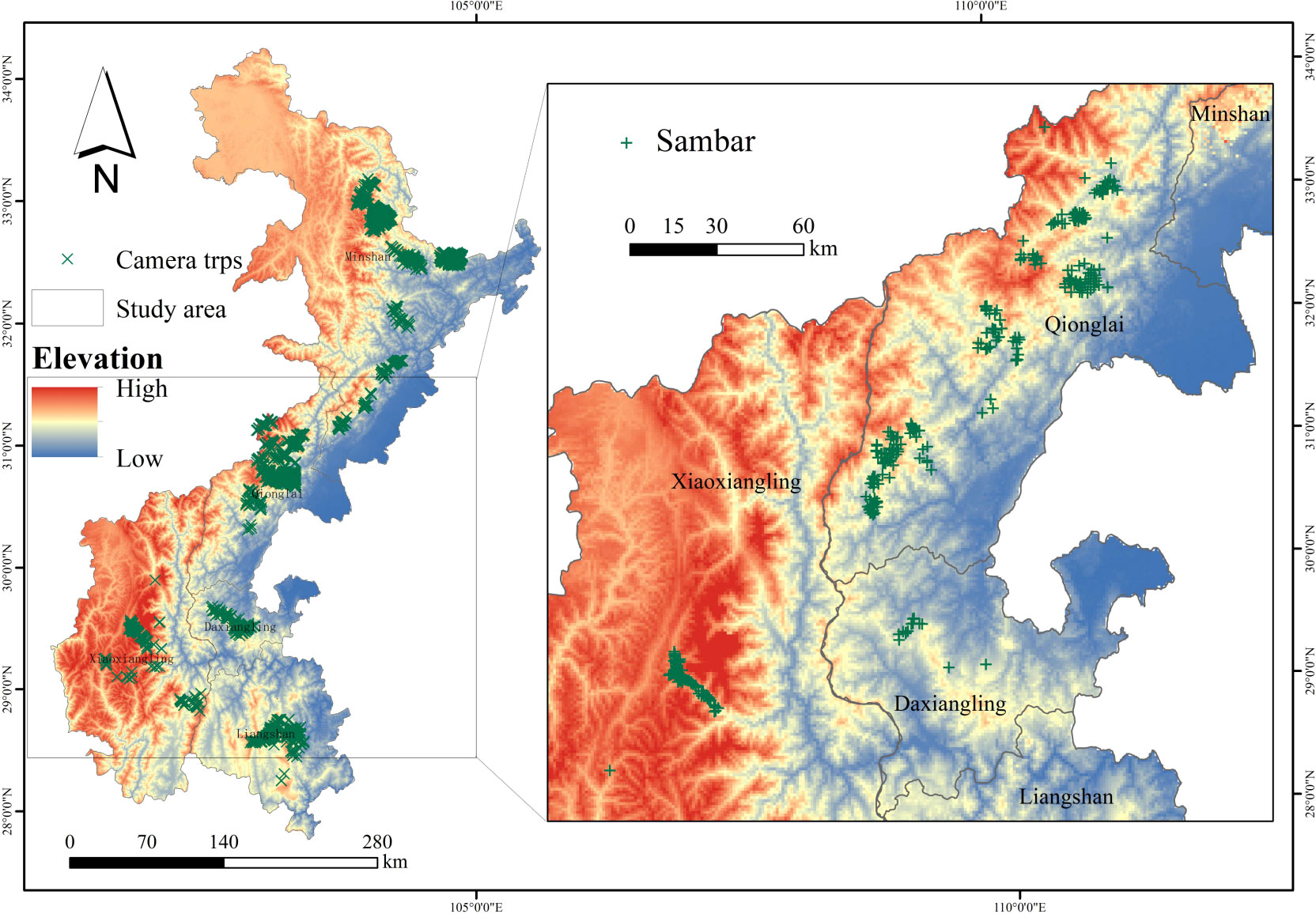
Front. Conserv. Sci., 19 January 2023 Sec. Animal Conservation Volume 3 – 2022 | https://doi.org/10.3389/fcosc.2022.909072
The next GIS application I examined was Impacts of spatio-temporal change of landscape patterns on habitat quality across the Zayanderud Dam watershed in central Iran. This study uses GIS to analyze how land use and land cover have changed over time and how those changes affect habitat quality. I focused on the habitat quality maps, which show areas ranked from low to high quality. Darker colors on the map indicate higher habitat quality, while lighter colors represent more degraded habitats.
I noticed that areas closer to urban development, agriculture, and the dam itself showed lower habitat quality over time. In contrast, regions farther from human activity, especially natural and undeveloped areas, tended to maintain higher habitat quality.

Phillips, S. J., Anderson, R. P., & Schapire, R. E. (2006). Maximum entropy modeling of species geographic distributions. Ecological Modelling, 190(3-4), 231–259. https://doi.org/10.1016/j.ecolmodel.2005.03.026
Quiz: Taken.