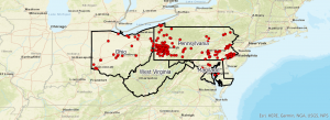
Author: amstratton

Chapter 4-

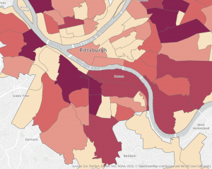
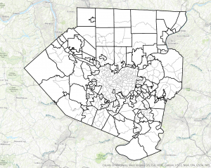
This chapter was about mapping density. I learned that you would use this to show highest concentration of features are, and to look at patterns rather than locations of the individual features. It eases viewing of maps with higher concentration as well. You map density two ways, either create a density surface or create a map based on features summarized by defined area. In a map based on features summarized by defined area, it would be mapped graphically, with a dot map, or just by calculating density value for each area. This method is easy buy doesn’t show exact centers of density, especially in large areas. Density is treated as a ratio with this method. Dot maps could be used when you’re mapping individual locations summarized by defined areas, and they show the density graphically. With a dot map you map each area based on total count or amount, and specify each dot value. This method is used when you already summarized by area or for comparing administrative or natural areas with defined borders. When you’re graphing a density surface, you use a raster layer and each cell gets a density value based on the number of features in the cell. The density surface method is precise, but requires more data processing.  This method is used when you want to see the concentration of point or line features. The GIS in this method will define a neighborhood around each cell center, and total the number of features that are in the neighborhood then divide that number by the area of the neighborhood. It then creates a running average of features per area. When calculating density values, you can do it based on cell size, search radius, calculation method, or units.

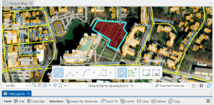
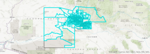
Chapter 5-

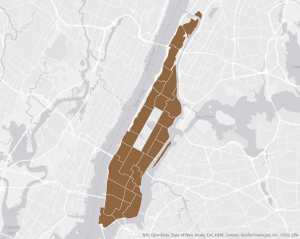
This chapter overviews how to tell what features are within a given area. You would map what’s inside to monitor what’s occurring within the area or to compare multiple areas on what’s inside of them. Monitoring areas allow people to know when to take action on the features within, and comparing areas will tell where there is more or less of something. You would draw an area boundary on top of the features and select the features inside and summarize them. When looking at a single area, you can monitor the info with several ways. These include; a service area around a central facility, a buffer that defines a distance around some feature, an administrative or natural boundary, an area you draw manually, or the result of a model. Multiple areas are for comparing, they could be contiguous, disjunct, or nested. This chapter also explains the three ways to find what’s inside; drawing areas and features, selecting the features inside the area, or overlaying the areas and features. Drawing areas and features are good when you want to see whether one or a few features are inside and out of the area and is created showing the boundary of the area and the features. Selecting the features inside the area is good for getting a summary of features inside areas and finding out what’s within a given distance of  a features and it’s created by specifying the area and the layer containing the features. Lastly overlaying the areas and features is good for finding which features are in each of the several areas or how much of something is in the areas, and it’s created by combining the area and the features ot create a new layer with the attributes of both or by comparing the two layers to calculate summary statistics for each area.

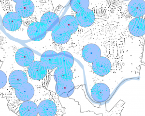
Chapter 6-

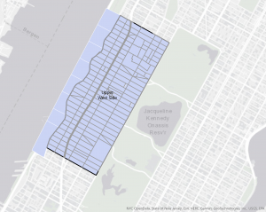
This chapter is about spatial proximity and nearness queries in GIS. It explores how to define, measure, and interpret what is near in a geographic context. To find what’s nearby, you can measure straight-line distance, measure distance or cost over a network, or measure cost over a surface. You can measure nearby based on a set distance, or on a travel to or from the feature.  Measuring using cost for example is how much time it takes from one feature to another. There are three ways to find what’s nearby; straight line distance, cost over a surface, and distance or cost over a network. For Straight line distances, you specify the source feature and the distance and the GIS will find the area or surrounding features. For cost over a surface, you specify location of the features and a travel cost and the GIS will create a new layer showing the travel cost from each feature. Lastly for distance or cost over a network, you specify the locations and a distance or travel cost along each linear feature and the GIS finds which segments of the network are within the distance or cost.

Chapter 7-

In this chapter I learned how to move, rotate, and add and move vertex points of a polygon, as well as adding polygons. When adding the polygons in 7-2, I had trouble finding the coordinate system the book wanted me to use, I scrolled through all of them for like 20 minutes until I finally found it. The rest of the chapter taught me how to smooth the polygons and make the polygons more intricate and detailed.

 

Chapter 8-

This chapter works with zip codes, and  collect events. The second tutorial is this chapter taught me how to build a street locator and geocodes.

 

Chapter 9-

This chapter I learned how to use the Pairwise buffer tool to create buffers around features, as well as finding the sum of features. I also learned how to create a multiple ring buffer and stats related to the features within the buffers, and also creating a gravity model.

 

Chapter 4-

This chapter I started to have a really fun issue, where I couldn’t run ArcGIS Pro on my desktop directly. It would continuously try to have me redownload it, so the only way I could open the software was through the tutorial files. So in order to complete tutorial 4-1 and 4-2, I had to open tutorial 4-3, and access the “create new project” option through there. I was confused on the shapefiles in 4-1, because they would keep disappearing when I added a new one, but then I learned you had to click open a new tool to save it. I also had trouble in 4-2 with deleting rows in the tables. I had to select them all individually and delete them instead of holding ctrl like the book suggests.  I kept getting error messages while trying to calculate the PercentPopYouth20 field, so I ended up skipping that part of the tutorial because it was frustrating me.

Chapter 5-

In this chapter, the first tutorials were simple, just teaching me different projections of the maps.  On the third tutorial everything went fine, until i went to change the coordinate systems to what the book instructed and it wasn’t there so I ended up skipping the California map.

 

Chapter 6-

In this chapter I learned how to use the pairwise dissolve tool to create neighborhoods.  Then I learned how to isolate different study areas using different “select by” tools. I also learned how to merge separate features using the “merge” tool, as well as adding features using the “append” tool. This chapter went very smoothly for me.

\

Zip Code: All the zip codes in Delaware County, updated monthly. 

School District: All the school districts in Delaware County.

Building Outline 2023: All the building outlines in Delaware in 2023.

Street Centerlines: The center of pavement of roads in Delaware County.

Address Points: All the addresses in Delaware County. 

Parcel: All of the cadastral parcel lines in Delaware County.

Condo: All of the condominiums in Delaware County.

Subdivision: All subdivisions and condos in Delaware County, updated daily and published monthly. 

Recorded Document: All points of recorded documents in Delaware County, such as surveys and annexations. 

PLSS:  All the Public Land Survey System polygons in both the US Military and the Virginia Military Survey Districts of Delaware County.

Township: All 19 Townships in Delaware County. 

Dedicated ROW: All designated Right of Way lines in Delaware County.

Precincts: All voting precincts in Delaware County. 

Delaware County E911 Data: All certified addresses in Delaware County. 

Building Outline 2021: Building outlines for all structures in Delaware County in 2021.

Original township: Original townships in Delaware County before the tax districts changed the shapes.

Map Sheet: All map sheets in Delaware County.

Farm Lot: All farm lots in US military and Virginia Military survey districts in Delaware County.

Annexation: All annexations and conforming boundaries 1853-now in Delaware County. 

Survey: Survey points that represent land surveys in Delaware County. 

Tax District: All tax districts in Delaware County.

Hydrology: All major waterways in Delaware County. 

GPS: All GPS monuments from 1991 and 1997. 

 

Chapter 1-

This chapter taught me basically how to navigate the software, like how to access different tabs and what they’re used for, and creating or using bookmarks .

 

Chapter 2-

I had some issues figuring out how to apply the labels at first, but eventually I got there once I realized I have to wait until after the settings are done to click the label button. Overall didn’t have too much trouble with anything else, and was able to go through the tutorials smoothly.

Chapter 3-

This chapter had me working with layout, charts, and how to create these maps to be easily readable for people who don’t regularly work with maps or aren’t familiar with the topic or area you’re mapping. It also taught me how to share maps to ArcGIS Online. I had some issues sharing it, because none of my files would show up in the files explorer, it would just tell me that my “container is empty”. Consequently, I couldn’t find the tags or summary box fields to complete. I ignored that and still shared both maps. I had no trouble navigating the ArcGIS Online portion of this chapter.

 

Chapter 1

Chapter one gives a basic overview and an introduction of what GIS is, and how it is used. GIS is a process that looks at geographic patterns in data and relationships between features. This chapter lays out the steps to starting the GIS analysis process; frame the question, understand your data, choose a method, process the data, and look at the results. There are three types of features, discrete features, continuous phenomena and summarized by area. Discrete features are locations that can be directly pinpointed. Continuous phenomena is measured anywhere and covers entire areas, like temperature or rain. Lastly, features summarized by area represent numbers or density of an entire area. There are two ways to represent these three features, vector (typically used with discrete and data summarized by area) and raster (usually used with continuous phenomena). The chapter then goes over briefly how map projections distort shapes and measurements, and advises that small areas can ignore the distortion but it’s more of a concern when mapping larger areas like states or countries. There are five geographic attributes that help describe features, categories, ranks, counts, amounts, and ratios. Categories are groups of similar things that organize and make sense of the data, like categorizing roads as freeways or highways. Ranks are putting features in order, from high to low when measures are difficult or a combination of factors. Counts are numbers of features on a map and amounts represent any measurable amount of things associated with a feature. Ratios represent the relationship of two quantities by dividing one by the other. Lastly the chapter overviews how to use data tables that hold attribute values and summary statistics. There are three common operations, selecting, calculating, and summarizing. 

 

Chapter 2

Chapter two goes into detail about making a map using GIS, and what they could be 

used for. Mapping features can show patterns in the distribution of those features, and start to find the causes of those patterns. The chapter describes the process of making a map, starting with patterns from the data you collect and mapping those features with symbols. You have to think about the audience that will be viewing the map, adding reference locations to give context to the analysis or to make it more recognizable, and how the map will be presented, changing information presented based on size scale. Another thing it reminds you to do is make sure there are geographic coordinates assigned to the features you’re mapping. To map a single type of feature you would use the same symbol, and the GIS stores the locations of the features as a pair of coordinates that define its shape, so it can draw the features with the symbols you choose. To map by category, you would draw the features with a different symbol for the different category values, and the GIS stores each value for the features. You can also use many different categories to show other patterns in the data sets, but using more than 7 categories can make them much more difficult to see. The larger the area, the smaller number of categories would be beneficial and vice versa. Grouping a large number of categories can make it easier to see the patterns as well, as long as you’re specific about what the categories include. When choosing symbols, choose based on the type of feature. Individual locations would use a single marker in a color or shape for each category and linear features would get different variations of lines, and shaded or raster layers get different shades of the same color. 

 

Chapter 3

Chapter three describes mapping most and least values. You would use mapping most and least when you want to go beyond just mapping locations of features and give your audience more information about your data. You would map patterns of these features that have similar values, and the quantities associated with the three types of features discussed in chapter one, discrete, continuous phenomena, and data summarized by area. You assign symbols to these features based on their attribute (also discussed in chapter one, counts, amounts, ratios, and ranks), which contains a quantity. Counts and amounts show you total numbers, and lets you see values of the features. This is only a good method for discrete features and continuous phenomena because it would skew the patterns for summarizing by area. Ratios even out the differences between large and small areas, areas with many or few features, to give a more accurate distribution of said features. It’s very useful when using the summarizing by area type of feature. Ratios could be; averages, for comparing a place that has few features against one with many, proportions, showing part of a whole quantity and what it represents, and densities, for showing where features are concentrated. Ranks are useful when direct measures are difficult or for combinations of factors. The chapter also overviews how to create classes when using counts, amount and ratios, because each feature has a different value. There are four common standard classification schemes for grouping classes, natural breaks, quantile, equal interval, and standard deviation. Natural breaks, also known as Jenks, are based on natural groupings in your data and breaks where values jump. Similar values go in the same class. Quantile classes include an equal number of features in each class. Equal interval classes show the difference between the high and low values as the same for each class. And lastly, standard deviation classes are based on how much their values vary from the mean. The chapter then goes over how to compare each class, and the advantages and disadvantages for each one.