Author: amhickman

Data 1: PLSS – This is a feature layer, PLSS meaning Public Land Survey System. It was created to facilitate the PLSS and boundaries for the US and Virginia Military Survey Districts of Delaware County It is updated on an as-needed basis

Data 2: Township – Feature Layer: This shows all the townships that are in Delaware County.

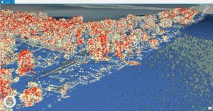
Data 3: 2024 Aerial Imagery: Spring 2024, planes flying over Delaware county in spring

Data 4: Delaware County E991 Data – Feature Service: This map shows the 991 emergency response, accident reporting, geocoding, and disaster management in Delaware County. It helps 911 agencies comply with phase II 911 requirements

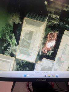
Data 5: Building outline 2021 – Feature Layer: This shows the outlines for all the structures in Delaware County in 2021, when it was last updated.

Data 6: Original Township – Feature Layer: This is a map of what the original township boundaries were. This was before tax district changes affected township shapes.

Data 7: Zip Code – Feature Layer: All the zip codes in Delaware County are in here. Tax-exempt parcels were added by whichever zip codes they were most related to.

Data 8: School District – Feature Layer: This contains all the school districts in Delaware County. It was created by the Delaware County Auditor’s parcel records of the school districts.

Data 9: Building Outline 2023: Same as Data 5 but for year 2023.

Data 10: Recorded Document: A map that shows all the recorded documents in the Delaware County Recorder’s Plat Books, Cabinet/Slides, and Instruments Records.  Some of these documents include ones containing vacations, subdivisions, centerline surveys, surveys, annexations, and miscellaneous. It is updated weekly and posted monthly.

Data 11: Dedicated ROW: Contains all the lines that are designated as right-of-way in Delaware County. They are stores within Delaware County Recorder’s office. There are currently 1256 records.

Data 12: Subdivision: This contains all subdivisions and condos in Delaware County. Currently 5917 records.

Data 13: Address Point: Represents all the certified addresses in Delaware County. There are currently 113797 records.

Data 14: Map Sheet: Shows all the map sheets in the county.

Data 15: Farm Lot: This shows all the farmlots that are in both the US and Virginia Military Survey Districts of Delaware County. 2077 records

Data 16: Annexation: This shows all the annexations and conforming boundaries since 1853. 421 records

Data 17: Survey: This represents the surveys of land in Delaware County. Old survey volumes 1-11 are not included. 17848 records

Data 18: Tax District: This shows all of the tax districts in Delaware County. 61 records

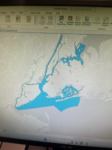
Data 19: Hydrology: This shows all the major waterways in Delaware County. It was enhanced in 2018 with LIDAR-based Data. 24 records

Data 20: GPS: This shows all the GPS monuments in Delaware County. 351 records

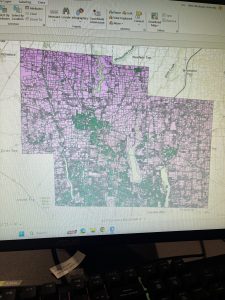
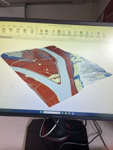
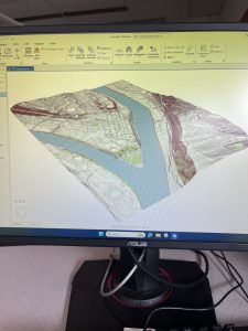
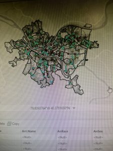
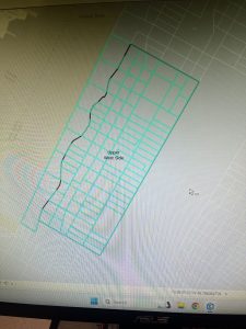
Here is a screenshot of center streetline, hydrology, and parcel:

Chapter 9:

In Tutorial 9-1, I had some trouble with the tables. I only got the number of youths within 0.5 miles of a public pool. I did not get the other numbers. Tutorial 9-2: I couldn’t find output fields or the merge rule. I was completely confused for tutorial 3, but I breezed through 4.

Chapter 10:

While doing tutorial 2, the Threshold would not show up, I did everything it said to do. In 10-3, I couldn’t calculate the field for ZFHHCHLD. I kept getting an error.

Chapter 11:

I really liked chapter 11, specifically tutorial 1. being able to really see all the aspects in a different view rather than one map view was nice.

Chapter 4:

As I started tutorial 1, the Tracts feature under youth population in the catalog pane was not appearing. As I could not find the Tracts feature, I also cannot do tutorial 2 in Chapter 4 as it requires the tracts feature… I, however, can start on Tutorial 3. In tutorial 3, I was supposed to get 444 remaining, but I got 430. In tutorial 4, I was very easily able to complete it. I liked when I was able to add color at the end for the choropleth map.

 

Chapter 5:

I liked being able to see the globe in a different perspective. In tutorial 3, I had trouble finding the “NAD 1983 UTM Zone 11N”. It was in a different spot than what the book referred me to. I ended up finding it however. My favorite part of this chapter was adding another baselayer. It is cool to see the different parts of areas.

 

Chapter 6:

Chapter 6 was the easiest for me. I liked being able to see just the specific parts of areas. Here are a few pictures of what I got.

 

Chapter 7:

This chapter was fun. I went crazy fixing all the building polygons. It was lowkey driving me insane that they were all a bit off.

 

Chapter 8:

I was a bit confused with this chapter, but I got a bit of it understood, like the first part.

Chapter 1:

I found Chapter 1 to be relatively easy, but also a bit confusing as this was my first time using GIS software. I found it interesting that it chose Allegheny County out of everything as that is where I’m from.

 

Chapter 2:

My favorite part of chapter 2 was being able to change the colors of the different areas like water and parks. There were so many varieties of colors that could be chosen. Obviously, the book wanted us to use specific colors though.

 

Chapter 3:

I found this chapter a bit confusing. When I got to it, there were certain parts that I learned in chapters 1 or 2 where it expected me to remember what to do. It was fun making the different graphs and everything though,

Chapter 4: Identifying Clusters

Chapter 4 explains how to identify clusters, which happen when features are found in close proximity. By pinpointing, it can help to determine cause of clusters in that particular location. Statistics are used to determine if there are reasons for the clusters or if they happened by chance. Cluster of features with similar attribute values can be brought up using discrete features, spatially continuous data or data summarizing. They are interval or ratio values. Depending on what you are trying to pinpoint, you may have to put a specific period of time, or even a specific date. Clusters are almost always defined by straight-line distance. This could work, unless you are trying to find distance in travel time. The nearest Neighborhood hierarchical clustering specifies the distant features that can be found from each other in order to pbe part of a cluster. It also determined the minimum number to be able to consider it a cluster. It can also show the clustering at different geographical scales. To see the orientation of individual clusters, GIS may calculate the standard deviational ellipse for the points. To find the causes of clusters, you would want to compare clusters to a control group. To do this the control group and clusters can be mapped together, or you can creat clusters for the control group and compare them with the original clusters being analyzed. Clusters can also be identified on whether they are similar to their neighbors or not. Basically, if high values are surrounded by high values, they were similar, and vice versa. Using Moran’s I, means you are interested in local variation. A large positive value for Moran’s I indicates that the feature is surrounded by features with similar values, and a negative value means the feature is around dissimilar features. The G-statistic shows where cluster of high and low values are. There are two different methods. The Gi statistic helps you determine the effect of the target feature and what is going on around it. Gi* is the where you can find hot and cold spots.

Chapter 5: Analyzing Geographic Relationships

Chapter 5 begins with examples of how GIS is used in different fields. Some of the fields mentioned were transportation analysts, environmental lawyers, archeologists, state police, and wildlife biologists. In stats, attributes are the variables. Two analyze the relationships between attributes, you can use a defined area, sample point, or raster cell. The variables from different layers need to be associated with the same geographical unit. A ratio needs to be used if the locations are two different sizes. For different sets of features, they need to be combined somehow. To do this, you can either do a polygon layover or create rasters of the areas, making them the same size. Variables can also be created to represent spatial interaction between features. These features could be distance, travel time, or travel cost. Statistics is a huge thing when coming to analyzing geographic relationships. spatial autocorrelation is one. It violates the assumption that observations are independent. It brings the redundancy into analysis. To study the relationship between two variables as well as the nature, you measure the extent to which they vary together. Values have a direct relationship is the they both increase when one of the also increases. If one decreases while another increases, that is an inverse relationship. Other than that, there won’t be a relationship. There are also posiitive and negative correlations.

Chapter 1:

One of the first things Chapter 1 mentioned was statistics. It can take large amounts of data and summarize it into small segments, for example, geographic analysis. It can help you find unknown values from values that have already been derived. Statistics has not always been used in GIS software until recently, when programs like CrimeStat and Spacestat started coming around. Using spatial statistics can help to find patterns in geographical locations. You can also find where those patterns are located on a map. You can also find if different features can relate to eachother. An example from the book was the relationship between the quality of infant health in relation to the neighborhoods across a country. Infant health may different in different neighborhoods. Chapter 1 also mentions different areas of work, like geostatistics to be able to study air pollution and soil contamination. To be able to start a geographic analysis, you need to know what information you are looking for. To be able to do this, you have to assume that the opposite of your hypothesis is true. After finding the data you want to use, you need to understand it. This means looking for a location and deciphering whether it is dicrete or continuous. Discrete means lines, points or areas. Continous feature are temperature and precipitation. Using summarized data will give you a the data of an entire area, rather than a specific location. There is nominal, ordinal, interval, and ratio data. Nominal data are features of a similar type. Ordinal data is as it says ordered. It can be either from high to low or low to high. Interval data tells you the regular magnitude. Ratio data is the relationship between two quantities. Interval data and ratio data go hand in hand, both being continuous. You will also need to choose a method, and then calculate the statistics. Once you find the significance of the statistics, you will also have to quation the results. An example the book gives is the idea of straight-line distance and the travel time when defining how close these features are to each other.

Chapter 2:

Chapter 2 is the measuring of geographic distributions. You can use GIS to find the center of a statistical distribution. The center is the extent to which featured are clustered or dispersed. The center can change depending on. the direction of the dispersion of the cluster. Sometimes the characteristic you are trying to find may not be apparent, which is when you would calculate a statistic. I liked the example of the crime analyst for comparing the distributions of different features. One way would be mapping the dispersion of auto thefts, assaults, and other thefts to see how the distributions occur. The crime analyst was also used as an example for tracking change. If they want to see the differencei n burgluries during the night and day, they watch the center for a few months for each night and day. There are three kinds of centers. The mean center is when there is no travel to and from the center. A median center is where you need to find the best location for something. It could be a location that is the shortest distance to all other locations, also known as a central feature. A central feature is the shortest total distance from the other features. The center can be found by location alone, or by an attribute value. An unweighted center is use for incidents that occur at a certain place and time. The weighted center is calculated for stationary features.  The median and central feature are calculated using the distance between the features in the data set. An outlier can skew the mean or median centers. The less features there are, the more an outlier could skew. “The standard distance measures the extent to which the distances between the mean center and the features vary from the average distance”(42).

Chapter 3:

Chapter 3 helps to identify patterns. Two ways to identify patterns is either by displaying the features or values on a map or using statistics to measure the extent of the clusters. The results would be tested to calculate the probability that the pattern did not happen by chance. Using the statistics method is more accurate. Local statistics can help find hotspots in a global statistic, however, sometimes global and local do not agree. Quadrat analysis is used when there is no direct interaction between features. The nearest neighbor index measures where the nearest neighborhood is to a feature, and then calculates the average. I feel that would be good for real estate when they are trying to sell houses and computing the nearest town to a neighborhood. The quadrat analysis measure the density of features, but not the proximity or arrangement between them. Two tests used to test the results of the quadrat analysis is the Kolmogorov-Smirnov Test and the Chi-square test. The Kolmogorov-Smirnov test calculates the proportions of quads for each line in a frequency table, as well as, the running cumulative total of the proportions. The chi-square is used to find the difference between two sets of frequencies.

 

In all, I think chaoter 3 was the most interesting. I have taken a statistics class in the past and this chapter made the most sense.

Hello! I’m Ariauna Hickman. I’m from Pittsburgh Pennsylvania. I’m a sophomore, majoring in Pre-Professional Zoology on the Pre-Veterinary track. I am also double minoring in business and chemistry. A quick fun fact is that I have a Great Dane who is a goofball.

After reading Schuurman ch. 1, it is clear to see how important GIS is in many different career choices. I like how it can be used for many different things. The part where it mentions how municipalities use it for things like affects on highways, however, confuses me a bit. How are they able to tell how it affects those areas? Now that I read the next page, my question was answered. It is to see how it would work with landscapes and housing. It is crazy to think about how more than 50% of our brains neurons are used for visual intelligence. No wonder GIS is so important. It is like a visual way of seeing geographical locations. The visuality is used as a means to be able to make it more accessible to see the patial awareness of areas.

After looking at a few different ways that GIS is used. I found how it can be used for video games.  For example, Watch Dogs 2 usesGIS in the way that it is open world. They made it highly detailed and realistic with the urban planning, architecture, and digital infrastructure. GIS is also used in Pokemon GO. People go around using a geographical map that matches their location to go and catch different pokemon. It is a blend between the physical and digital world.

Geographic Information Systems, Intersections, Iowa Computer Science Education Week 2023, Technology, Video Games, Video Games and GIS, Wael Alhaj