Chapter 4. 4-1. This section is about making a geodatabase. These are useful since you can continuously add data to them, and they have no limit to the amount of feature data that you can add to it. To start, make a new project map, then add the data that you need, in our case it is the Maricopa County folder. To add this navigation to the contents pane and click folders then add folder connection and select the folder you want to import. To accrual use the data in the folder we imported we had to convert a shape file (an old file type) to a feature class. To convert from a shapefile to a feature class go to tools in the analysis pane, then select the export features tool. There are other export tools that can be used to convert different types of files (like CSV) to tables (Export tables). Note that to turn off a layer in a geodatabase you need to delete the feature, you can not simply turn it off like in the contents pane.
4-2. To create a new column in a data table right click the feature class, go to its attribute table, click options, then fields view. Add a new field, then save. It will likely have no data in it so go back to the attribute table then right click the new column, then calculate the field. In the calculate field pane double click the data you want to be imported to that column then ok. To join tables, right click your desired feature layer, then click joins and relates, then add join. This join is not permanent so in order to make it stick right click the layer you have been using this whole time, then click data and export features. This converts the table that was made into a feature layer.
4-3. This section has us using attribute queries which allows us to select data rows and spatial features based on the values we tell it. This is similar to the SQL we did in the previous week. We have to use a script to do our query and some key things to know are: text values need to be in “”, number values do not need to be in quotes, most of the time an or statement needs to be in parentheses. To display only features that we want from a class, use select by attribute and use the expression you want, then open the attribute table for said layer, then go to properties for that layer and make a definition query and use the same expression you use to select, then click ok. This displays only the features you want displayed, and this can be verified in the table. To make an “or” expression with the definition query write out your expression and then click the SQL editor button to see the actual script, then add parentheses around the or statement. We used attribute selection to observe the amount of burglaries on weekends vs. weekdays. This was done by using a definition query to select the month of august and the crime type and attribute select to filter the days of the week. We selected Saturday or Sunday, and then in the attribute table we can use the switch button to select all the weekdays and back; allowing us to see the distribution of weekend and weekday crimes
4-4. This section teaches us how to use the spatial join tool. This tool allows you to join the spatial data from 2 feature classes into 1. To do so just locate the spatial join tool and select the layers you would like to join together.
4-5. Creating central point data for polygons generates a point that is in the middle of a polygon. This is done by using the calculate geometry attributes tool, selecting your input field, then using 2 fields of X and Y with the central point as X, and Y coordinate respectively. This is a good way to generate graduated symbols since they are centred.
4-6. This section is about creating a table for data that is hard to interpret or understand called one-to-many data, which includes terminology or codes that untrained people likely cannot interpret without a reference (i.e. police or FBI codes). To join the table with the data, right click the point layer with spatial data, then select joins and relates, then add join.
Chapter 5. 5-1. This chapter is about spatial data, specifically how coordinate data is interpreted and generated. There are different types of spatial data projections that are useful at different scales due to the curvature of the earth. The standard coordinate projection that is used for GIS is GCS WGS1984, but it is not good at showing real spatial distribution, so instead we used Hammer-Aitoff world to show the globe, which shows distribution rather well at a global scale. This is done by right clicking the base map and going to properties, coordinate systems, projected coordinate system, world, and then Hammer-Aifoff.
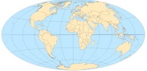
Hammer-Aitoff world map projection.
5-2. It is good practice to visualize projections that show good area, over shapes and angles. A good projection to use for the continental United States is Contiguous Albers Equal Area Conic.
5-3. When choosing a projection for the United States check the livingatlas website for your study areas code. This helps to choose a projection that is best for your region that has the least amount of distortion. This section also includes how to add data to a map, this is done by clicking add data under the map tab and selecting the data you want to add.
5-4. There are many ways to store data, and many file types. Some of the most common for shape files are .shp, .dbf, and .shx. Those files are for geometry, attribute tables, and indexes of spatial geometry respectively. To convert a shape file to a table just like with feature classes, use the export features tool, then right click the table and select create points from table, then select current map under coordinate system. To convert KML data to a feature class, use the KML to layer tool.
5-5. This section has us downloading US census bureau data and using it to make our map. To get started go to census.gov/cgi-bin/geo/shapefiles, choose a year, and layer type. Then further census data can be downloaded from data.census.gov. To format the data in XL we made columns: GEO_ID, MALE_BIKE, and FEMALE_BIKE for our commuter census data.
5-6. To add data from the living atlas, go to the catalogue pane, then select portal, then living atlas. This allows you to use data from the web, in our case we accessed the NLCD which shows national land cover usage. We then used the extract by mask tool to create a mask that only shows the raster data in Hennepin county. In the extract tool, in the environment under the extent tab I used the current display, and then the extent of layer buttons to select Hennepin county. Contour data and other types of data can be found at apps.nationalmap.gov/downloader.
Chapter 6. 6-1. This chapter deals with dissolving block groups and aggregating polygons. To dissolve block groups use the pairwise dissolve tool.
6-2. This section teaches us how to create a study region using multiple layers with an abundance of features. To display only a region from a layer, use the select by attribute function to select your designated space, then go to data for the layer containing said feature, then click export feature and create a new layer. Then to select data within your exported feature you can use the select by location button to designate the layer you want to select data from and where you want that to be localized. To clip 2 layers together, use the pairwise clip tool, this allows you to select data within a given area.
6-3. To merge multiple layers into one use the merge tool.
6-4. To merge points from 2 datasets into one, use the append tool, the target dataset is the one where all the points are going and the input datasets are where the data is coming from.
6-5. To generate a layer that has lines or points intersecting a given set of data, requires the use of the pairwise intersect tool.
6-6. To create a layer that has set data that is combined from 2 other layers, use the union tool.
6-7. The tabulate intersection tool can be used to associate data with different classes, such as assigning a split amount of disabled persons to different fire companies.