Month: September 2025

Chapter 4: 

Adding a folder through the Catalog pane enables you to access and import data from that folder into your current project.
Older shapefiles can be converted into feature classes, ensuring they can be fully utilized within ArcGIS. ArcGIS provides tools to create, modify, or delete fields in a feature’s attribute table, as well as apply Python expressions to manipulate the data they contain. By joining tables, you can extract only the information relevant to your analysis from a larger dataset. With SQL queries, you can filter datasets to locate only the records you need, using search terms combined with Boolean operators. Spatial joins make it possible to count the number of features within a defined boundary and generate the results as a new layer.

Chapter 5:

Because the Earth is spherical while maps are typically displayed on flat, two-dimensional surfaces, different map projections are used to translate the 3D surface onto a 2D plane—each with its own strengths and limitations. The Robinson Projection is commonly used for general purposes when displaying the entire globe. No matter which projection is chosen, the larger the area being represented, the greater the distortion that will occur. In GIS software, shapefiles are a widely used format for storing vector data. Many sources of spatial data are freely available online, allowing you to download only the datasets that are relevant to your project. Esri’s Living Atlas provides access to extensive collections of geospatial data, which can be added directly to your project using the Add Data tool.

Chapter 6

GIS provides tools to aggregate data by dissolving or combining smaller groups into broader categories. The clip tool allows you to reduce a larger dataset to a specific region, aligning it more closely with the focus of your project. Multiple datasets can be appended together to form a single, larger feature class. The union tool enables you to merge two polygon feature layers into one combined output layer.

Chapter 4

• database- container for the data of an organization, project, or other undertaking for record keeping, decision-making, analysis, or research
  • geodatabase is Esri’s database for geospatial data

Tutorial 4-1

• software automatically creates geodatabase when you start an ArcGIS project
• can connect to other folders for easy access
• shapefile- spatial data format for a single point, line, or polygon layer
• 

Tutorial 4-2

• much of what is displayed by GIS depends on attributes- columns of data in tables
• you can download data from external sources (ex: US Census Bureau) to map
• added a column to Tracts attribute table
• 

Tutorial 4-3

• GIS links tabular data to spatial features in feature classes
• SQL criterion: attribute name <logical operator> attribute value
• 

Tutorial 4-4

• count burglaries by neighborhood
• created choropleth map based on the join count I added

Tutorial 4-5

• GIS creates central points when you use graduated colors for symbology for polygon layer
• created fields to find coordinates of central points
• Feature to Point calculates central points instead of centroids

Tutorial 4-6

• creating code table and necessary fields/data

Chapter 5

• learn about latitude and longitude coordinates and their geographic coordinate system
• map projections- making flat maps from the nearly spherical earth

Tutorial 5-1

• Longitude: 0-180 east to west
• Latitude: 0-90 north to south
• 100+ map projection in GIS
• graticule- networks of lines on the map (30-degree intervals east-west and north-south)
• changed map shape
• 

Tutorial 5-2

• working with US map projections
• Albers equal-area standard projection for US Geographical Survey (USGS) and US Census Bureau for US maps
• larger part of world you need the more distortion

Tutorial 5-3

• Foe medium/large scale maps use localized projected coordinate systems specific to the study area
• need to use a reference map to determine what zone you are in to apply the correct coordinate systems
• adding layer adopted new coordinate system to the map

Tutorial 5-4

• review file formats for vector spatial data
• GPS and many other databases provide coordinates with x,y values
• KML is the file format used to display geographic data in many mapping applications (international standard for Open Geospatials Consortium)
• 

Tutorial 5-5

• use data from US Census Bureau
• learned how to clean up data in Excel
• trying to export files into the ArcGIS crashed my computer and I had to restart it and couldn’t finish the tutorial

Tutorial 5-6

• rasters are large files and should probable be stored elsewhere
• 
• Bicycle Count Stations wasn’t there where it said it would be

Chapter 6

• geoprocessing- framework and set of tools for processing geographic data

Tutorial 6-1

• 

Tutorial 6-2

• workflow for creating study region from layers that have more features than needed
• created feature class from selected features

Tutorial 6-3

• merging water features into a new single layer
• 

Tutorial 6-4

• use Append tool to add features to an existing feature class
• Added FireHouses and PoliceStations to the attribute table

Tutorial 6-5

• intersecting features to determine streets in company fire zones

Tutorial 6-6

• Union tool overlays geometry and attributes of two input polygon layers to generate a new output layer
• 

Tutorial 6-7

• 

Chapter 7:

I learned how to change the size of the outline and rotate it.

I also learned how to add and move vertex points. 

Lastly I learned how to delete different polygons.

Chapter 8:

In this chapter I learned how to use geocode data by zip code. 

I also learned how to rematch attendee data by zip code. 

Lastly I learned how to geocode street addresses. 

 

 

 

Chapter 9:

In this chapter I learned how to use buffers for proximity analysis. 

I learned how to spatially join service areas and pool tags. 

Lastly I learned how to be able to perform data cluster analysis.

 

 

 

 

 

 

 

Chapter 4:

• Adding a folder through the catalog pane allows you to import data from that folder into your current project
• Older shape files can be converted to feature classes in order to fully utilize them in arcgis.
• Arcgis allows you to selectively create, modify or delete fields within a features data table and use python expressions to manipulate the data held within them.
• Joining data tables together allows you to select only the data you need for your application from a much larger set.
• Sums, averages, concatenations and many other operations can all be completed on data fields using Python expressions.
• Using SQL queries, data can be sorted through to find only the information relevant to your search by using search terms along with boolean operators.
• Spatial joins allow you to count the number of a feature within a bounding region and output it to a new layer.

Chapter 5:

• Since the earth is a sphere, but maps are usually displayed on a 2D surface, various map projections are used to translate the 3D surface onto a 2D one, with various drawbacks and advantages to each
• The Robinson Projection is best for general uses where the whole earth needs to be shown
• The larger the region you are trying to display, the larger the amount of distortion that the map will have, no matter the projection used
• Shapefiles are a common data type used for vector data in GIS software.
• Spatial data can often be found and downloaded for free on the internet, allowing you to select only the data you need for your project.
• Living Atlas gives you access to large quantities of geospatial data that you can download directly into your current project through the add data button

Chapter 6:

• GIS allows you to aggregate data by dissolving or combining finer groups into more general ones
• You can clip a larger map down to a single region to more closely match the focus of your project
• You can append data sets together to create a single larger feature class
• The union tool lets you combine two polygon feature layers into a single output layer

 

 

Saving Project Name

 

Project (next to map,insert, analysis, etc tab) → save project as

 

Name Tutorial number Name.aprx

 

Displaying a Map

 

Bookmarks→map of choice

 

Basemaps

 

Basemaps = layers for what you wish to represent (rivers, topography, etc)

 

Contents Pane

 

View + Pane = select contents 

 

Contents = selector for what layers you wish to eliminate and keep 

 

Catalog Pane

 

 View tab → windows group → Catalog Pane

 

Allows for easy access to all project components

 

Export Layer tool

 

Share tab (after project, map, insert, etc under the logo in left top corner) → export layer

 

Saving Images

 

1. On the File Type drop-down menu, click PNG.

 

1. For Name, click the Browse button, browse to save the file to your top, and rename it FQHCAndUrgentCareClinics.png.

 

150. For Resolution, type 150.

 

1. On the Color Depth drop-down menu, click 24-bit True Color.

 

1. Click Export to run the tool.

 

T: 1-2 Navigating Map Display

 

Navigation of Map

 

Map tab→full extent→explore button = center map/info on features

 

Bottom right buttons do things

 

Wheel button Zooms in 

 

Map Back button

 

Map tab→Navigate→ arrows

 

Turing all Feature classes on/off = ctrl on press hold + check box click = on/off for all

 

Bookmarks

 

Bookmarks = zooms to thing you select

 

Creating new bookmarks = bookmarks (navigate) + new bookmark + name

 

Manage bookmarks = bookmarks (navigate) + manage bookmarks

 

Selecting Attributes data = Right clicking + attribute table + select by attribute = where + Name + is equal to + location 

 

 

 

CHAP 4:

•  Works with spatial databases and databases in general
• You can open folder connections in the right click menu under folders, which will let you access the files without having to locate them every time
• there is a geoprocessing tool which can make a shapefile into features called “Export Features”
• Databases can be inputted from .csv files and be made copied and such in the catalog tab
• You can populate fields with the Calculate Field tool
• GIS synthaxing is in python script
• Attribute queries help one search database information
• The Spatial Join tool is cool and useful

CHAP 5:

• The grid on the first map is called a graticule and is 30 degrees intervals
• You can add projects to a spatial map – whats the difference between a projection and a bookmark?
• You can look up the coordinate system of the USA on ArcGIS’s living atlas- what coordinate systems would I need to know for the rest of the world?
• You can download census data to use for GIS projects pretty easily on the gov’s website and other stuff on living atlas

CHAP 6:

• You can use the dissolve block group to separate blocks into specific neighborhoods
• You can clip attributes to areas to better study a specific area
• You can intersect features

Chapter 7:

• In this chapter, I learned how to trace, select, and move, and rotate polygons. 
• I learned how to add vertices under the edit tab.
• The lasso tool is used to drag vertices and change the polygon shape, and the split tool is to split a polygon. 
• Creating a polygon: On the Edit tab, in the Features group, click Create. In the Create Features pane, click the desired feature, and confirm that Polygon is selected. On the Configure toolbar, with the Line button active, click to add points and draw a feature outlining the polygon. Double-click the last vertex point to finish the polygon.
• Delete polygons also using the delete button in the edit tab after selecting the polygon you want to delete. 
• Use the trace tool to create a polygon feature: On the Edit tab, click Create, and turn Snapping on. In the Create Features pane, click the layer you want and then the Trace button.
• Use the smooth polygon tool when creating the vertices of a new path. A shorter length will result in a more detailed (or smoother) path but will take longer to process.
• Transforming polygons: Turn off the base map layer. Then with the features you want selected, on the edit tab in the features group, click modify. In the Modify Features pane, click the Transform button. Under transformation Method, click Similarity 2D, and click Add New Links. Then, draw lines from vertices to where you want to move your polygon to. 

Chapter 8:

• Create locator -> put in appropriate fields -> run (geocodes survey data). In the Catalog pane, expand Locators, right-click the layer you want, and click Properties. Click Geocoding Options, and expand Match Options.
• Rematch addresses: In the Contents pane, right-click Attendees, click Data, and click Rematch Addresses.
• Symbolize using the Collect Events tool: Search for the collect events tool, apply settings, and run the tool. 
• Geocode addresses -> fill in fields -> run (converts addresses to geographical locations).
• There was very little in the tutorials for this chapter, mainly just geocoding, looking at attribute tables, and sorting data. 

Chapter 9:

• The pairwise buffer tool dissolves interior lines of overlapping buffers, merging them into a single buffer.
• Buffer rings create concentric zones around input features. (Multiple ring buffer tool).
• This chapter had more spatial join tool practice.
• Making a scatterplot example for this tutorial: In the Contents pane, select Polygons_Tags_Pop. On the feature layer’s Data tab, in the Visualize group, click Create Chart > Scatterplot. In the upper left, above Contents, click Chart Properties. In the Chart Properties pane, for X-Axis Number, click AverageTime; for Y-Axis Number, click UseRate.
• On the Analysis tab, in the Workflows group, click Network Analysis > Location-Allocation. Click the Location-Allocation layer tab. In the Input Data group, click Import Facilities, and apply necessary settings. Click Import Demand Points, and apply necessary settings. In the Travel Settings group, for Direction, click Towards Facilities, and type x amount for Facilities. In the Problem Type group, for f(cost, β), click Exponential. For β, type 0.25, and press Tab. Run the model. For this tutorial, this is how specific pools were located (by cost efficiency).
• Data Cluster Analysis: Multivariate Clustering tool -> apply settings -> run the tool.

Chapter 4:

This chapter focuses on classifying with different types of methods, symbology, and labeling. The different types of classification affect the way the patterns show up on the maps. We also learned about ways to make the maps cleaner such as basemaps, techniques for labeling, and transparency. The goal was to turn the information into readable on the map.

Chapter5:

Locating data accurately through coordinate systems was a main point of this chapter. Address locators, geocoding, and adding x,y data tables to make features was introduced. Aligning layers properly was also an important topic.

Chapter 6:

This chapter gave us ways to answer spatial analysis questions through buffers, overlays, and proximity tools. These were used to study spatial relationships between each other and the features. Differnt spatial and attributes were compared this helped me to understand how both data and geography can be used to filter information and answer questions. 

 

Chapter 4

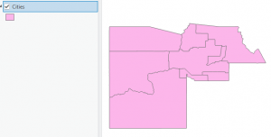
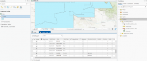
4-1: Importing data, setting up a folder connection, converting a shapefile to a feature class, importing a data table into a file geodatabase, and using database utilities.

• This was all fairly straightforward, but I was glad to familiarize myself more with the folder structure, as I’ve never really used folders outside of this class before.

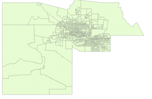
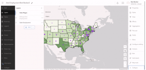
4-2: Deleting unneeded columns, adding a field and using the Calculate Field tool, joining a data table to a feature class attribute table, exporting a feature class, calculating a sum of fields, calculating percentages, and extracting fields.

• Again, this chapter was pretty easy, but I did struggle with deleting unneeded columns at first because I couldn’t find the “Delete” button. Overall, I thought that this subchapter included some pretty useful features that have very modern applications. 

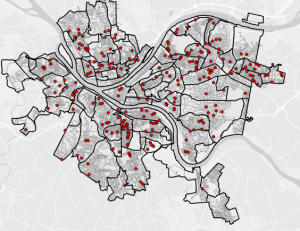
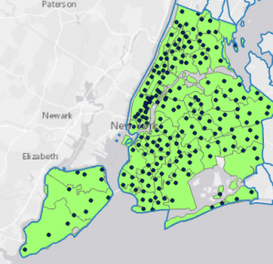
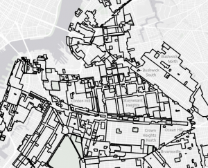
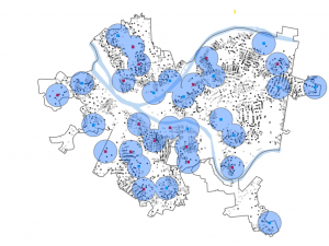
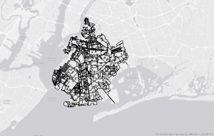
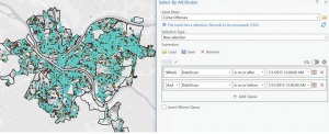
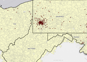
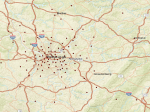
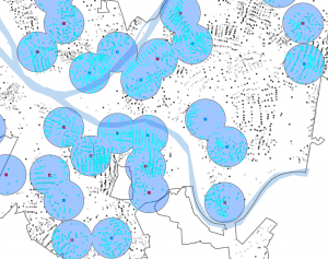
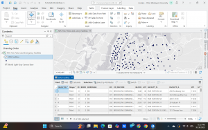
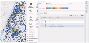
4-3: Viewing crime incidents, creating a date-range query, reusing a saved query, using OR connectors and parentheses, day-of-week range, and querying person attributes.

• This was probably my favorite subchapter so far, because I felt like a detective or something like that, trying to find crime statistics and locations of certain crimes. Using actual code was something new that I learned, although it was pretty basic coding. 

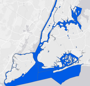
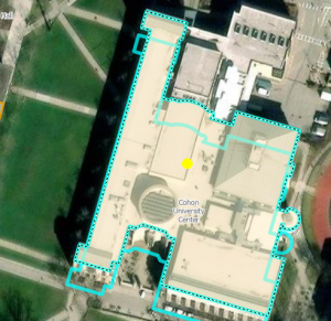
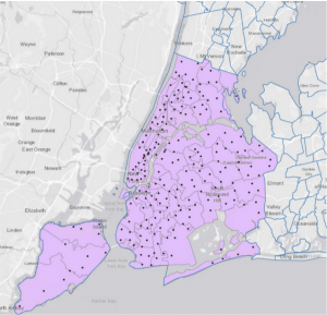
4-4, 4-5, 4-6: Building a spatial join, creating a central point feature class, creating a point layer, and making a one-to-many join.

• These subchapters were all pretty straightforward, although I did run into some trouble with the Calculate Geometry Attributes tool, and was a little confused on the formatting, but I figured it out in a few minutes. 

Chapter 5

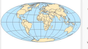
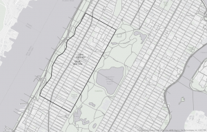
5-1, 5-2, 5-3: Using coordinate systems

• This was also pretty useful information, as I was able to change the way that the map was oriented and focus on different locations and regions. I had no issues with these subchapters. 

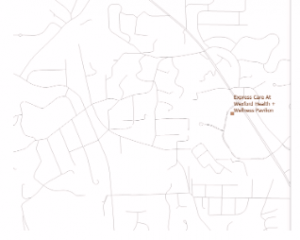
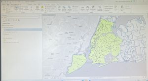
5-4: Shapefiles, adding x,y data, converting KML files to feature classes.

• This subchapter was a bit more complicated, as I am still familiarizing myself with files and other computer features, but it didn’t take me too long to figure it out.

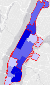
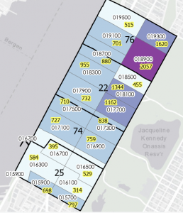
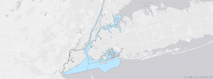
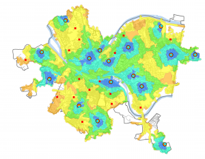
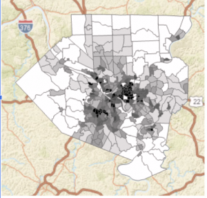
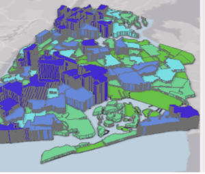
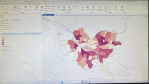
5-5: Downloading census data and files, processing data in microsoft excel, adding data to ArcGIS, and joining data and creating a chloropleth map.

• This subchapter was very hard for me, and I ran into a lot of problems using excel spreadsheets and downloading census data. The first time that I downloaded the Commuting Characteristics by Sex table, not all of the data was displayed in the spreadsheet, so I had to troubleshoot and redownloaded the data following the steps more carefully. 

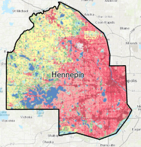
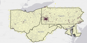
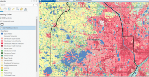
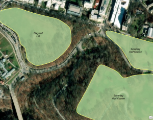
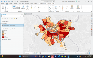
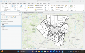
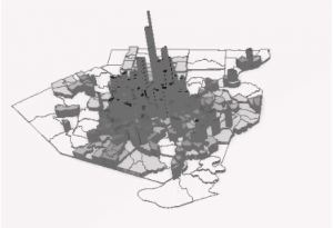
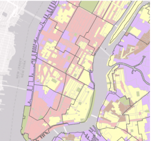
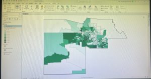
5-6: Adding a land use layer, extracting raster functions, downloading contours from a government organization, and downloading local data from a public agency hub.

• I liked this subchapter (and the previous one, excluding the issues I had) because it used data from Hennepin County in Minnesota, which is where I am from, so it was cool to apply GIS to something that relates to me. I didn’t run into any of the issues like in 5-5, but it took me longer as I was very careful in following the instructions to download data correctly. 

Chapter 6 (Disclaimer: I completely forgot to take pictures of my work from this chapter, and will edit this post with pictures the next chance I get)

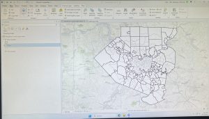
6-1: Dissolve fields and dissolve block groups.

• This was all pretty straightforward, but I did struggle a bit with the “Your turn” section as I had to retrace my steps from the first portion of the subchapter and was confused on exactly what to put in the input and output fields. 

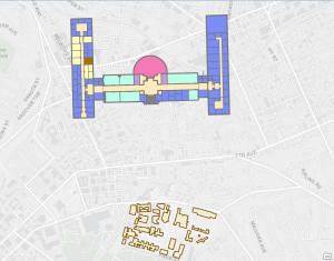
6-2: Creating a study area, creating study area block groups, and clipping streets.

• I had no issues with this subchapter, as I am familiar with all of the features.

6-3, 6-4: Merging features, and appending features.

• The merge and append tools were very easy to use, and I had no issues. 

6-5: Intersecting features, summarizing street length.

• This was all pretty straightforward, and I found the tools to be very useful.

6-6: Calculating acreage, and summarizing residential land-use areas.

• This felt similar to some of the previous subchapters, almost repetitive at this point. 

6-7: Using tabulate intersection.

• This was something new, but I found the tool pretty easy to use.

Chapter 1

• ArcGIS- integrated collection of geographic information system software developed by Esri

• ArcGISPro- 64-bit desktop GIS application that uses a ribbon interface for 2D and 3D mapping

• Feature class- basic building block for displaying geographic features on a map

• • • Homogenous layer on map
    • Vector data with corresponding attributes for each feature

• Raster dataset- major type of spatial data that is a picture made up of a bunch of pixels

• File geodatabase- with extension.gdb that stores feature classes, raster datasets, and other related files

• Project- file with extension.aprx that contains one or more maps and related items

• Basemap helps orient users to location
  • ex:

• Catalog pane provides access to all components in ArcGIS project
  • Can create map with heading through this

Tutorial 1-2

• Learned how to find attribute data for a feature
• Learned how to zoom in on feature
  • 
• Spatial bookmarks allow you to zoom to preset map views
• Can right click feature to get attribute table

Tutorial 1-3

• Can change order of attributes, names and displayed names of attributes, see data types, delete attributes, and make only certain attributes visible
• Learned more about how to navigate attribute table

Tutorial 1-4

• Learning how to change symbols for feature classes (color, shape)
• Explored 3D maps
• 

Chapter 2

• Thematic map- consists of a subject layer/s (theme) placed in spatial context with other layers
• Make subject prominent while placing spatial context layers in the background

Tutorial 2-1

• Context layers often displayed using outlines with no color fill
  • Water features exception- blue color, no outline
  • 

Tutorial 2-2

• Learning how to label all layers of map
• Learned how to filter out duplicate labels

Tutorial 2-3

• Use definition query to limit features to a desired subset of the larger collection based on values in feature attribute table
• 

Tutorial 2-4

• Choropleth map- uses color in polygons to represent numeric attribute values

• • Use classification methods to display data (default method is natural breaks)
    • Uses algorithm to cluster values of numeric attributes into groups
    •  

Tutorial 2-5

• Learning to display polygon data in their centers

Tutorial 2-6

• Choropleth map showing population useful for studying needs like demand for goods and services
• Choropleth maps of normalized data provide different data than choropleth maps of total population
  • Normalized = segment of population divided by total population
• Density maps also form of normalized maps
• Can import and reuse symbology

Tutorial 2-7

• Dot density maps can be used to denote quantitative values
• Display a total number randomly across a statistical unit

Tutorial 2-8

• Visibility ranges automatically turn layers and labeling on and off, depending on zoom
• Small scale- 1:50,000,000
• Large scale- 1:24,000
• Can turn a feature layer on or off using visibility ranges

Chapter 3

Tutorial 3-1

• Building map layout that has two maps
• Had some troubles here loading second map
• Learned how to add legends beside maps
• Because of struggles displaying the second map, I wasn’t able to follow the instruction for the create charts section

Tutorial 3-2

• Learning how to publish and share ArcGIS maps online
• Learning how to access our maps using ArcGIS Online
• I realized I have been signed into somebody else’s ArcGIS Pro this whole time…
• 

Tutorial 3-3

• Learned how to create story on ArcGIS Online
  • Added various headers, subheadings, paragraph texts, and maps
  • 

Tutorial 3-4

• Dashboards- visual displays of data feeds in an easy-to-understand format, usually with map as center of focus

• Learned how to create a dashboard
• Had issues filling screen with map, so I couldn’t finish the very last part