Address Point
A comprehensive and spatially accurate dataset of all certified addresses within Delaware County, Ohio. This dataset is updated daily and made available on a monthly basis.
Annexation
Tracks changes to municipal boundaries in Delaware County, including annexations and territorial adjustments since 1853. Updates occur as needed when changes happen, with monthly publications.
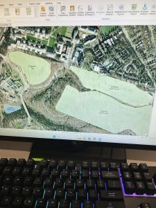
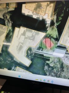
Building Outline
Outlines the physical structures across Delaware County.
2021 Dataset: Last updated in 2021, with updates occurring as needed.
2023 Dataset: Last updated in 2023, with updates occurring as needed.
Condo
A dataset containing all condominium properties in Delaware County, represented as polygons.
Dedicated Right-of-Way (ROW)
Contains all designated road right-of-way areas in Delaware County. This dataset aligns with parcel data updates and is updated as needed, with monthly publications.
Delaware County Contours
A topographic dataset displaying two-foot elevation contours across the county, based on 2018 survey data.
Delaware County E911 Data
Utilizes the Address Point dataset to determine the closest emergency response location for any given address. This dataset is updated daily and published monthly.
Farm Lot
Identifies the locations of farm lots throughout Delaware County. Updates occur as needed when new surveys are conducted.
GPS Monuments
A record of established GPS control points (monuments) throughout Delaware County, used for geospatial referencing.
- Last updated in 2021, with updates occurring as needed.
Hydrology
Maps major waterways, including rivers, lakes, and streams. The dataset was last enhanced in 2018 and is updated as needed.
Master Street Address Guide (MSAG)
Maintains a record of all official street addresses in Delaware County, along with their respective jurisdictions (cities, townships, and villages). Updates occur as needed.
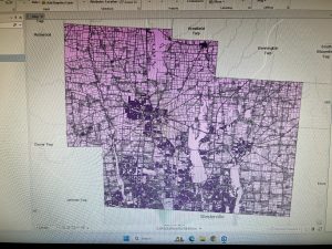
Map Sheet
Contains all official map sheets for Delaware County.
Municipality
Defines and maintains the boundaries of all municipalities within the county.
Original Township Boundaries
Displays the historical township boundaries before modifications due to tax districts. This dataset remains unchanged over time.
Public Land Survey System (PLSS)
Contains land division information based on public land surveys, including those conducted by the U.S. Military and Virginia Military surveys. Updated as needed, with the latest update on February 28, 2025.
Parcel Data
Includes all land parcel boundaries within Delaware County. Maintained by the Delaware County Auditor’s GIS Office, updated daily, and published monthly.
Voting Precincts
Outlines all voting precincts within Delaware County, maintained by the Board of Elections and updated as needed.
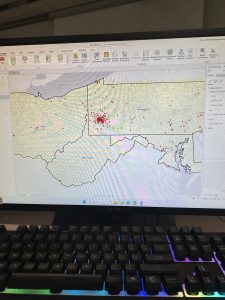
Recorded Documents
A dataset containing points linked to recorded property-related documents within Delaware County. Updated weekly and published monthly.
School Districts
Defines the geographic boundaries of all school districts in Delaware County. Updated as needed.
Street Centerline
Represents the centerline of all public and private roads in Delaware County. Used for transportation planning, emergency response, and accident reporting. Updated daily.
Subdivision
Records all subdivision developments and condominium communities. Updated daily and published monthly.
Survey Data
A dataset showing locations of land surveys conducted throughout Delaware County. Maintained by the Map Department, updated daily, and published monthly.
Tax Districts
Defines tax district boundaries in Delaware County, maintained by the Real Estate Office. Updated as needed.
Township Boundaries
Shows the defined borders of the 19 townships in Delaware County. Updated as needed and published monthly.
Zip Code Data
Represents the ZIP code boundaries within Delaware County, refined using postal and census data.