Month: January 2025

Chapter 4:

This chapter talked about file geodatabases (FGDBs), which allow a large storage capacity and better performance in ArcGIS Pro. Before I read this chapter, I hadn’t fully understood the importance of FDGBs. Coming from a Biology background (before I changed my major to Computer Science), I initially thought of spatial data like large Excel datasets. Here spatial databases have geographic features, which makes them more complex than a simple table. Some cool things that I learned were that FGDBs allow fast queries and spatial relationships. This reminds me of databases in bioinformatics. In addition, I learned that FGDBs store multiple layers efficiently. Before, I thought shapefiles were enough. I now understand how limited FGDBs can be. They allow better organization, which makes them much needed for GIS. If I see a .gdb folder I now know that it means that it holds many classes, raster datasets, and tables. This chapter provided us with hands-on tutorials, showing us how to create geodatabases and how to import shapefiles. One of the tutorials showed us how to collect spatial data, like when it summarized crime incidents by neighborhood. As a Data Analytics major, I found it interesting how similar GIS queries are to data analysis tasks that I have done in Excel. This tool seemed more powerful, as you can filter data based on more stuff. Python is very valuable for ArcGIS and I would love to explore its use more. Some questions that were raised was if FGDBs have limits for large environmental datasets. Another question that I had was how can Python automate file geodatabase tasks in ArcGIS.

 

Chapter 5:

 

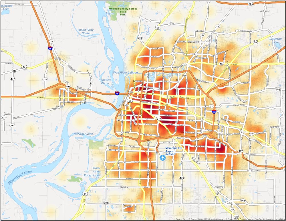
Before starting to learn GIS, I never thought about how maps can reveal hidden patterns. After reading this chapter I now get their importance and how powerful tools they are. This chapter talks about mapping an area. This is necessary as we can understand what is going on inside the mapped area. For example, where the highest crimes happen in a city, or which hospitals are within 5 miles of schools, etc. Instead of looking at raw data tables– which can be overwhelming most of the time- GIS successfully condenses and summarizes this data. I was familiar with latitude and longitude, but I had now idea about map projections and coordinate systems. I feel like I am learning a new language when I try to understand spatial data. I understood how easily things can go wrong if I don’t choose the right projection. I finally understood why some maps deform distances. Another interesting thing I learned was vector and raster data. I related raster data to a microscope image, as there are grids and pixels that have different intensities. From the tutorial, I saw that if I choose the wrong coordinate system the datasets will be completely misaligned, and that would ruin the analysis. As someone who hated high school geometry, I never thought that I would enjoy working with coordinate systems. The real-world applications made me appreciate GIS even more, as it showed me how important it can be for making decisions. I also learned that spatial data interoperability is how different data get to work together. Some questions I have are how does datum transformation affect GIS precision?

 

Chapter 6:

 

This chapter showed us that knowing what is near you is important for making decisions. Whether it’s finding the closest hospital or analyzing wildfire risks. GIS plays a fundamental role in spatial decision-making. I really liked how practical this chapter was. Geoprocessing tools allow you to repeat and automate GIS workflows without having to click through the menu. Some key takeaways from this chapter were the dissolving features, like merging school districts into larger administrative regions, clipping data, and merging datasets. The last one is essential when we have to deal with large environmental datasets. Lastly, spatial intersections, which for me was mind blowing. I liked how you can overlay two datasets and extract the affected area. What really stood out to me was geoprocessing. It is used by emergency services to assign fire stations to fire zones while making sure that the response times are the desired ones.  In addition, straight-line distances are the shortest way possible between two locations. It can be simple, but can also be considered unrealistic because there are a lot of factors that should be taken into consideration, like how people are actually driving, sidewalks, crosswalks, etc. GIS isn’t just about mapping, it is about solving real-world problems. A question that I had was how geoprocessing scales with large data sets, like would it slow down?  Another one was how GIS combines road issues and other things that must be taken into account in order to calculate and analyze locations more accurately. This chapter made me think about how much GIS impacts our everyday life without even knowing it. From finding what is the fastest way to go somewhere, to emergency responses. A final thought that I had when finishing this chapter reading was that I felt more confident about ArcGIS Pro. In the beginning, I struggled with what GIS is and what is its use, but now I am getting it

Chapter 4

The first thing that really grabbed my interest when reading this chapter is how the mapping of density looks visually. That might sound kinda dumb cause that is the whole point of GIS, but I believe that the gradient looking mapping of density plays exceptionally well, at least to my, towards our sense of what the data represents. I find it quite easy to interpret the difference between the darkly shaded areas of density compared to the lighter shaded areas that surround it, representing less density. To contrast this though, I’m not the biggest fan of how the use of dots to represent density appear on maps. In the section about dots it shows a map before and after using them for density and to be honest the one that JUST represented each individual business was far easier to read. Funnily, the dot system (not for density) seems to be very helpful to be but beside and used with a density surface map, showing the finder details of whatever data you’re projecting.  Within all of this and the idea of density I feel like I’m reading a lot about computer calculations and stuff which is confusing, just really wondering how much of this stuff I only kind of understand needs to be known well. I know I’ve absolutely said this before a few times in my last journal, but there is definitely a disconnect between me and the specific knowledge that I need to be gaining in order to complete this course when we go to the Application. I will note though that I’ve just heard that part week 5 is hard and I’m probably overthinking the severity of this little issue.

Chapter 5

(What I’m writing here was wrote before I finished the chapter, but isn’t this kind of just everything overexplained. Like if there was nothing inside your map it just wouldn’t be there.) I hate to go back to the old classic immediately, but this chapter feels like it’s not really conveying any new information to me without using GIS along with it to see what its talking about. Like it still feels weirdly obvious that you should be able to locate and see specific data in a specific area, I just still don’t exactly know how to do that myself. It feels like someone is trying to teach me how to shoot a basketball, but he wont show me how to do it and just tells me all the ways to do it right. Yes, that is helpful, but at least for me it would be a lot better to actually see and work on the shot.

Chapter 6

From what I understand this is just chapter 5 but about what surrounds specific things on the map instead of what specific things surround this are of the map. At this point in the reading I’m struggling very hard to figure out how to write more about any of this. I’m very much so at a point where there has been so many things that only kind of make sense to me piled up that its all kind of not making sense. However its weird because it’s also almost impossible to not understand it because a lot of what I am reading feels like its just saying the same basic idea of “you can see how far this is away from that” over and over again in slightly different ways. Like I know that I’ve read literally hundreds of pages about this, but the more I read the less it feels like I’m reading anything. I’m sorry if I may be being kinda picky about the reading or whatever, but I seriously don’t know how to write about any of this anymore. I’m at a point where it feels like there isn’t any more starter information to soak up through this book and that I am only getting more confused by the repetition of almost identical ideas. I know that especially for these last two chapters I really didn’t write much, but I cant figure out how to keep writing it. Big props to Andy Mitchel for being able to write all that!

Chapter 4 is all about mapping density. It discusses why it is important, the different ways to map density, how to map density for specific areas, and how to decide what to map. The definition of mapping density is where the highest concentration of features is. One thing that was very helpful was when the book explained that you should look at your features and the information needed to complete the map before making a decision on what kind of map to create. Density maps are also more helpful for comparing areas. There are two ways you can map density. The first is by defined the area using a dot map. Dot maps are beneficial for representing the density of individual things in large areas. The other use of dot maps is when you have many features in one space and don’t want to map all of them individually. The second way to map density is through density surface. This is created as a raster layer as opposed to a vector. It is more detailed than a dot map but requires more time and effort. The book goes on to lay out the comparisons and explain how to decide which mapping method to use. Then, it explains what GIS does and how that applies to mapping density, which I found very helpful. There are multiple factors that affect a density map, including cell size, which determines how “fine or coarse” the patterns will be; search radius, which determines how generalized the area the map is showing will be; calculation method, which will determine how clear/easy it is to interpret the map, and units which help make sure the map is accurate.  Something I had not considered important was the colors used on the map. It was interesting to read that while “more” on most maps is darker, the contrast of making “more” lighter colors can help grab the reader’s attention.

Chapter 5, titled “Finding What’s Inside,” is all about why it is important to map inside an area. The first examples the book gives are about whether or not one should take action based on the map’s findings. There are numerous questions to answer when analyzing your data before mapping. The first is how many areas you are planning to map, which can be determined by what it is that you are mapping. The second question is whether or not the features inside are discrete, meaning they are identifiable or continuous, which are seamless geographic features. There is also important information you must get when analyzing your data. You must determine how you get your information (count, list, or summary) and also determine whether to include features partially inside of the area. The book then highlights the three ways to determine what is inside an area. You can draw what’s inside the area, select the features inside the areas, and overlay the features and areas. The first is best for seeing if one particular feature is in an area. Selecting the features is best for getting lists or summaries, and overlaying is best for finding how much of something is in an area or seeing if something is in more than one area. One important thing this chapter highlights is how to make this kind of map easy to read. It talks about lines, locations, and discrete and continuous features. You can use the results from the map to make lists, and show statistics of features in that area. Overlaying areas is a useful tool to help find features and summarize them. Throughout the chapter, it highlights what GIS does in each feature and method listed which was helpful for me because it allowed me to understand the different uses of GIS better.

Chapter 6 is about finding something that is near a feature you are mapping. This is useful for finding out what is in an area’s traveling range or finding the specific distance between two features.  Similar to when finding what’s inside an area, you need to first define your analysis. A lot of the steps when finding things nearby are similar to the steps needed to find what’s inside. You should ask yourself many of the same questions and collect the same data. There are three ways to find what is nearby: straight line distance, where you identify the source and distance and then GIS finds everything surrounding it; distance over a network, which is when you explain the source and distance; and GIS finds things that meet those parameters, and cost over a surface which is when you declare what each source feature is and a cost and GIS creates a new layer on the map with each features cost. Another similarity between chapters five and six is that they both compare each method and explain when it is best to use each one. A term that comes up a lot in this chapter is buffer. A buffer is a zone a certain distance from the designated area in every direction. Buffers are important because yu can specify multiple sources and see the distance from each one of them and how they overlap.  There are different ways you can set up a map once you have a buffer depending on what you want the readers to understand from it. Instead of a buffer you can also select features at “x” distance. This is similar to a buffer but without the physical boundary/circle shown on the map. Another option when finding things nearby is “feature to feature” which will show you the distance between two features. The last option the book discusses in this chapter is creating a distance surface. This means creating a raster layer of all of the continuous distances.

 

The ESRI Guide to GIS Analysis, vol. 1  (second edition, 2020) by Andy Mitchell

Chapter 4

Density maps show where the highest concentration of features is and are particularly useful when looking for patterns in areas that vary in size, such as census tracts and counties. Before creating a map, the kind of data being used and whether the density of features or feature values will be mapped should be considered. Density can either be mapped graphically (calculating density values for each area or dot mapping) or by density surface. If the data have already been summarized by area or the objective of the map is to compare administrative or natural areas with defined borders, density should be mapped by defined area. If the objective of the map is to see the concentration of point or line features, a density surface should be created. When mapping density for defined areas, calculating a density value for each area involves dividing the total number of features/total value of the features by the area of each polygon while creating a dot density map involves specifying how many features each dot represents and how big the dots are. Density surfaces, however, are created in GIS using raster layers. The specified cell size, search radius, calculation method, and units affect how the GIS calculates the density surface and, ultimately, what the patterns will look like. Density surfaces can either be displayed using graduated colors (usually displayed using shades of a single color with common classification schemes including natural breaks, quantile, equal interval, or standard deviation) or contours (connecting points of equal density). While the patterns on a density map are partially dependent on how the density surface was created, it is important to remember that there may not actually be any features where the highest density is. To see a better picture of what is going in a place, the locations of features from which the density surface was calculated should also be mapped with the density surface or on a separate map.

Chapter 5

Mapping what is inside an area allows for the monitoring of what is occurring inside it or the comparison of several areas based on what is inside each. Depending on the number of areas, what type of features are inside the areas (discrete or continuous), and the information needed from the analysis (list, count, or summary), an area boundary can be drawn on top of the features, the features inside can be selected using a area boundary, or the area boundary and features can be combined to create summary data in order to find what’s inside. A map that shows the boundary of the area and the features is good for seeing whether one or a few features are inside or outside a single area. This method requires a dataset containing the boundary of the area or areas and a dataset containing the features. Creating a map by selecting the features inside an area is good for getting a list or summary of features inside a single area or group of areas being treated as one. A dataset containing the areas and a dataset with the features are needed for this method which involves specifying the area and the layer containing the features so that the GIS may select a subset of the features inside the area. To overlay the areas and features, the GIS either combines the area and the features to create a new layer with the attributes of both or compares the two layers to calculate summary statistics for each. Overlaying the areas and features is good for finding the features that are in each of several areas or finding out how much of something is in one or more areas. Data containing the areas and a dataset with the features are needed for this method. When selecting features inside an area, GIS can be used to create a report of the selected features (count, frequency, sum, average, median, standard deviation). There are also key differences between overlaying areas with discrete features, continuous categories or classes, and continuous values.

Chapter 6

What is occurring within a set distance or traveling range of a feature is understood through finding what is nearby. There are also three methods to find what is nearby: measuring straight-line distance, measuring distance or cost over a network, or measuring cost over a surface. Selecting a method entails determining the information needed from the analysis (list, count, or summary) and defining and measuring “near” which can be based on a set distance or on travel to or from a feature. Using straight-line distance means specifying the source feature and the distance before the GIS finds the area or surrounding features within the distance. This method is good for creating a boundary or selecting features at a set distance around the source. A layer containing the source feature and a layer containing the surrounding features are required to find what is nearby using straight-line distance. Using the area covered by segments of the network  within the distance or cost to find the surrounding features near each source is known as measuring distance or cost over a network. If the objective is to find what is within a travel distance or cost of a location using the locations of the source features, a network layer, and a layer containing the surrounding features, this is a suitable method. Measuring cost over a surface begins by specifying the location of the source features and a travel cost. Then, the GIS creates a new layer showing the travel cost from each source feature. This approach is good for calculating overland travel cost and it requires a layer containing the source features and a raster layer representing the cost surface. When calculating cost over a geographic surface, it is important to acknowledge that cost refers not only to monetary value but also to factors like time, effort, or resource expenditure required to traverse a landscape.

Chapter 4 centers around the concept of density and mapping it. Mapping density makes it easier to understand which areas are the most concentrated in some type of resource or landmark, for example in the book it references small businesses. Instead of simply plotting each location on a map where they could become overlapped and difficult to understand, you map with darker colors in areas of high density and include a key so that density can be better visualized. Mapping density rather than simply the location of features on a map gives you a measure of their density per area. Density can be mapped using a graph, a dot map, or calculating density for each designated area. Creating a density surface in GIS is usually preferable but it requires the most data input and more individual data on locations rather than data separated by region or county lines. GIS can also take a map density by area map and use the data to construct a dot density map to represent density graphically.
When using GIS to create a density surface there are many factors to consider including cell size, search radius, calculation method, and units of measurement. Another thing to consider when creating a density surface is that data that is summarized by defined areas can be used to make these types of maps but it must be generalized by the centroid of each defined area. This means that the summarized data is assigned to the point at the center of the defined area for which it is summarized. Additionally, for these maps a graduation of colors is assigned to each value so that the density can be visualized. The results of creating these types of maps in GIS are almost entirely dependent on the choices made with the many variables that can be manipulated in the program, meaning the same data can look different in final products where different visualization choices were made.

Chapter 5 discusses the need to map what is inside an area. This is necessary because the bonds for these areas can be “within 1000 feet of a school” or something like that to impose stiffer punishments on crime. This is an example of finding what is inside one area but you can also use mapping to find what is inside several areas such as each district in a city. In either case, you first have to know the boundaries of your area(s). Then, the discrete or continuous nature of the features you are measuring has to be taken into account. You can also use GIS to list features, count them, or get a summary. You also have to consider if the features being measured are completely in the area because discrete features can easily be partially in or out of a defined boundary.
There are three ways to find what is inside the area. First, drawing both the areas and the features, this way you can see the boundaries of your area and what features are inside it. This is specifically good if you only need to know which features are inside and outside of an area. Second, you can specify the area and the layer that contains your features so that GIS selects a subset of the features which is inside the area. This is best for getting a list of the features inside an area. Finally, you can overlay the areas and the features to create a new layer which compares the two layers and summarizes the statistics for each area. Which is best for doing both at the same time, as it is the most flexible.
Using the results of these summaries can be tricky. Some ways it can be used include: the count of a total number of features in an area, the frequency of a number of features with similar values in an area, or to summarize a specific numeric attribute such as the sum of certain features. These similar principles can be applied to much more complicated data, overlaying layers onto each other and creating understandable visualizations of complicated data over a range of areas.

Chapter 6 focuses on mapping what is nearby to a feature. This is important because some features may require notifying anyone living within a set distance. However, “nearby” is a concept that ranges in distance, within GIS you must define the distance which is being considered as nearby. Sometimes it is just straight distance away, or in some cases distance has to be measured using networks of transportation such as roads. Distance and cost can both be used to measure what is nearby, cost can include the amount of time it takes to get somewhere from your location. You also must consider the information you require from your analysis, sometimes it may be a list of everything “nearby”, a count of the total number of restaurants nearby, or a summary statistic for the area.
To determine “nearby” you can use GIS to set an inclusive ring based on straight-line distance, which is best for defining the area of influence around the feature. To do this you have to create a buffer in GIS at a certain distance from the feature you are discussing. Additionally, using this method you can use GIS to find the distance between two features, or to create a spider diagram with your chosen feature at the center. Another option is using distance or cost over a network (such as roadways), which is best used when measuring travel over a fixed infrastructure is necessary. GIS includes a ready-to-use street network which can be used to find whats nearby in terms of distance; however, this is not the only possible network you may want to use so custom networks can be built in the program. GIS will start at your feature and check the distance to the nearest junction in relation to your specified distance, and it will repeat this until a definition of everything “nearby” has been reached. You can also specify more than one center in this type of mapping. Finally, measuring cost (of time or another variable) over a surface is most helpful when you need to measure overland travel and calculate how much area is within your range. This has to be done using a raster layer of continuous distance from your feature.

Chapter 4: 

Chapter 4 dives into the concept of mapping density and its significance in identifying patterns and concentrations of features. Mapping density is especially useful for understanding patterns rather than focusing on individual features or locations. The chapter explains two primary methods of mapping density: by defined area and by density surface. In the defined area method, density can be represented using a dot map or calculated density values for specific regions. On a dot map, each dot symbolizes a fixed number of features, with higher dot concentrations indicating greater density. Additionally, shading areas based on calculated density values helps visualize where concentrations are higher or lower. The density surface method is more detailed and uses GIS to create raster layers, assigning density values to individual cells. This method requires more data and is time-consuming but provides higher accuracy, especially when analyzing specific concentrations. Each approach has its strengths: defined area mapping works well with pre-summarized data, while density surface mapping is ideal for examining specific points or locations. The chapter highlights that tools like dot density maps and raster layers simplify interpreting and visualizing density, enabling users to identify concentrated points or areas with ease.

Chapter 5

Chapter 5 emphasizes the importance of identifying and analyzing what exists within a specific area. Mapping what’s inside allows users to identify patterns, summarize features, and understand variations within different regions. This approach condenses complex data into accessible visual representations, helping viewers grasp where certain features or activities are more or less concentrated. The chapter differentiates between analyzing a single area and multiple areas. A single area provides focused, detailed insights, whereas multiple areas allow for comparisons across regions. It also highlights the need to classify features as either discrete (specific, countable items like buildings) or continuous ( less tangible elements like pollution levels). GIS tools offer three main ways to determine what’s inside: drawing areas and features, selecting features within an area, and overlaying areas and features. Drawing areas and features provides a visual representation of the data, while selecting features allows for summaries or counts of what exists within a boundary. Overlaying areas is especially useful for finding overlaps between features and regions. Overall, the chapter underscores the flexibility and efficiency GIS provides for analyzing what lies within specific boundaries.

Chapter 6: Finding What’s Nearby

Chapter 6 focuses on identifying features near a specific location and the methods for doing so using GIS. Understanding proximity is critical for planning and decision-making. GIS allows users to analyze what’s nearby by specifying a distance and then measuring that distance in different ways: straight-line distance, distance or cost over a network, or cost over a surface.The simplest method is straight-line distance, where you set a central feature as the source and define a radius to identify surrounding features. This is often used to create boundaries for proximity analysis. Another method is distance or cost over a network, which is useful for examining distances along roads or transportation networks. The third method, cost over a surface, focuses on analyzing travel costs across uneven terrain or landforms, such as overland travel. A key tool discussed in this chapter is creating a buffer, where you define a source feature and set a specific buffer distance. Once the buffer is established, you can identify, list, or summarize the features within it. Overall, this chapter builds on previous topics by emphasizing how GIS can analyze proximity, offering practical applications for planning and analysis based on what is nearby.

Chapter 1:

Chapter 1 focuses on an overall introduction to GIS. This introduction does not reduce GIS to ‘only a software,’ but also emphasizes the impact it has made across diverse disciplines. Through new technologies, researchers sharing their findings online, and advancements in the software itself, GIS has created a space for itself in disciplines from healthcare to construction. However, while this emphasis of the diversification of uses for GIS is important, what is more important is how the standard use of GIS has not changed. A user must still be able to structure their analysis properly and know which tools are applicable to the tasks they are carrying out. The part of GIS that has always interested me (without even knowing what GIS is) has been comparing mapping changes. Growing up in the rust belt in the early 2000s, much of what I remember as my hometown has been torn down. I remember neighborhoods upon neighborhoods of abandoned homes, however now even the streets they once stood on are gone. Chapter 1 goes on to expand upon what GIS Analysis is and the process of carrying it out. The portion under the subheading Frame the Question, “Or you may need to present results to policy makers or the public for discussion, for scientific review, or in a courtroom,” truly stuck out to me. I am currently taking Dustin’s Scientific Communication class. This concept of angling research and the language of said research to your audience is something that has interested me since beginning my undergraduate career. The way geographic features were described and explained was something that I cannot say I have ever seen before this reading. However, that being said I believe that these definitions are extremely valuable and should be introduced to those working outside the discipline of Geography/GIS. The skill of being able to read maps (both those for travel and information) is something that people my age are extremely lacking in. Taking these concepts such as ‘Discrete Features,’ or ‘Continuous Phenomena’ are elements of maps that I have often seen/heard of. However, this is the very first time I have ever been given a name to put to them.

 

Chapter 2:

As I’m reading through the first few chapters of this book, it is doing such a good job explaining these concepts that I often try to, but fall flat with my family/people outside of my major. It is very refreshing to see definitions that use simple language without diminishing content. The example, on page 24, of police mapping where crimes occur seems well intended, however, in practice wouldn’t this need exponentially more context and information? If implemented exactly how the example is written, could the GIS use be directly linked to potential over-policing? I appreciate the sections in the book where it is written in a way that prevents you from overthinking. For example, on page 26, it discusses using appropriate features, implying sometimes ‘less is more.’ Much of this chapter is introducing basic ‘rules’ to follow when mapping. Things such as creating multiple small maps if information is too compact, or choosing bright colors for important information and leaving more pastel/dull colors for necessary yet not critical info are themes that run strong throughout this chapter. All of this information, while it may seem lackluster or somewhat boring, is actually very crucial to making high quality legible maps. This portion of the chapter can also be related back to Dustin’s Scientific Communication class. In order to make your map as effective as possible, you must know your audience. A crucial part of ‘knowing your audience’ is changing the formatting of information without diminishing the quality of said information. In providing the reading multiple different examples of how to communicate the same information, the book is preparing future GIS users on adapting to their audience. One portion of the chapter that I am still not fully comprehending is the discussion of how GIS uses coordinates. I understand the basic premise discussed that you select the coordinates where you would like a symbol, to define boundaries of a land parcel, etc, however, are these coordinates that I have to retrieve on my own? If so, what is the process of doing so? I could be totally overthinking this (which would be a relief).

 

Chapter 3:

Chapter 3 keeps the focus on this set of ‘rules’ that are important to remember when making effective maps. However, where chapter 2 took a strict focus on the interpretability of maps, chapter 3 focuses on the quantitative aspects of these maps. Opening with the concept of mapping the most and the least, this first topic discusses how to successfully and efficiently communicate your numbers through the map. A very good example of this is the comparison between the mapped Locations of businesses vs. Businesses mapped by number of employees on page 52. The concept of Continuous Phenomena was somewhat difficult for me to grasp at first. I do believe that I was fully overcomplicating it for myself. However I still do have some questions about it. As continuous phenomena can be defined as areas or a surface of continuous values, how would I determine which is more effective? Is this something that I would just have to evaluate on a case-by-case basis? Am I thinking too much into this? Page 56 discusses the different ways that you can present this quantitative data and how this would impact the perspective of your audience. This portion of the chapter focuses on whether the use is ‘exploring the data or presenting a map.’ I have been consistently, pleasantly surprised by this book. I had assumed that these chapters were going to be boring, strictly informational pages discussing the actual usability of GIS. However, this approach of providing a user the practical, real-world uses for the software is very refreshing. It is getting me excited to stare at maps for hours on end. The section discussing counts, amounts, ratios and ranks was very helpful for me. As someone who does not have a brain for math, the explanation of what to use when was exactly what I needed.

Chapter 1:

In the first chapter of “The ESRI Guide to GIS Analysis,” Andy Mitchell introduces the concept of Geographic Information Systems (GIS). A GIS is a powerful tool that helps us understand and analyze spatial data information about the locations and shapes of features on Earth. The chapter begins by explaining the basics of GIS, emphasizing its role in transforming raw geographic data into meaningful information that can be used for various purposes. Mitchell discusses two main types of spatial data: vector data and raster data. Vector data represents features using points, lines, and polygons. For example, a point could represent a city, a line could represent a road, and a polygon could represent a park. On the other hand, raster data is made up of grid cells or pixels, and it is often used for continuous data like elevation or temperature. The chapter also highlights the importance of spatial thinking. It explains how GIS can be used to visualize patterns, relationships, and trends in geographic data. By using GIS, we can make more informed decisions in fields such as urban planning, environmental management, and disaster response. Overall, this chapter lays a solid foundation for understanding the fundamentals of GIS. It introduces key concepts and definitions that are essential for anyone interested in exploring the world of geographic information systems.

Chapter 2:

In the second chapter, Andy Mitchell focuses on the visual aspect of GIS. The chapter delves into the art of map design and the importance of creating maps that are both informative and pleasing. Mitchell emphasizes that good map design is crucial for effectively communicating geographic information. One of the key concepts discussed in this chapter is thematic maps. Thematic maps focus on a particular theme or subject area, such as population density, land use, or climate zones. These maps use various symbols and colors to represent different types of data, making it easier to understand and interpret the information. Symbology, the use of symbols to represent different types of data on a map, is another important topic covered in this chapter. Mitchell explains how choosing the right symbols and colors can enhance the clarity and readability of a map. He also discusses the concept of layering, which involves stacking multiple data sets to create a comprehensive map. By layering different types of data, we can gain a deeper understanding of the relationships and patterns within the data. Overall, this chapter provides valuable insights into the visual aspect of GIS. It highlights the importance of effective map design and offers practical tips for creating clear and informative maps.

Chapter 3:

The third chapter explores the process of interacting with GIS data through querying and selecting. Andy Mitchell explains that querying is a way of asking questions about the data to extract specific information. There are two main types of queries discussed in this chapter: attribute queries and spatial queries. Attribute queries are based on the characteristics or attributes of spatial features. For example, we might want to find all the cities with a population greater than 100,000. Spatial queries, on the other hand, are based on the location and spatial relationships of features. For instance, we might want to find all the parks within a certain distance of a river. Mitchell also introduces the use of Boolean operators (AND, OR, NOT) to refine queries and make them more precise. Additionally, the concept of buffering is explained. Buffering involves creating zones around a feature to analyze proximity and spatial relationships. For example, we might create a buffer zone around a highway to study its impact on nearby wildlife. Overall, this chapter provides a comprehensive understanding of how to query and select data in GIS. It offers practical techniques for extracting meaningful information from geographic data and emphasizes the importance of precision and accuracy in spatial analysis.

Hello, my name is Jake Marzulli I am majoring in Sports management and getting a minor in coaching. I love running and being outdoors and hanging out with my friends doing various activities Aswell as traveling to warm places!

Chapter 1

Chapter 1 of Schuurman’s book gives a fascinating overview of Geographic Information Systems (GIS) and how it plays an important role in our daily lives. GIS is more than just making maps it helps us understand patterns and solve problems in many fields like farming, government, and business. One interesting example is how scientists use visuals, like the double helix image of DNA, to figure out relationships and cause-and-effect. GIS does something similar by turning data into pictures that make it easier to analyze and make decisions. The part about farming really stood out. Farmers now use tools like GPS and soil analysis with GIS to figure out the best way to plant crops or deal with issues like blight (a crop disease). This helps them save time and money, but it makes me wonder if smaller farmers without access to this technology might struggle to keep up. It seems like technology could create a bigger gap between big farms and small ones. In cities, GIS is used in things like planning garbage collection routes, fixing roads, and creating bike paths. Schuurman shows how it makes life more efficient, but I liked the part about traffic jams during road repairs it’s a funny reminder that even advanced tools can’t solve every problem perfectly. The section on e-governance was also really interesting. GIS helps governments deliver services like registering cars or planning new parks. This can make things easier and fairer, but it also raises concerns about privacy. For example, governments collect a lot of digital data, and people might worry about how it’s used. Overall, this chapter shows how important GIS is for understanding and organizing the world around us. It’s not just about technology it’s about how we use it to shape our society.

First Gis Application

This article discusses how GIS helps police predict and prevent crimes by analyzing historical crime data and identifying hotspots. By visualizing crime patterns, police can allocate resources more efficiently, improving crime prevention and response times.
Source: The Times

Second Gis Application

This is interactive map where users can view reported incidents of various crimes, such as theft, assault, and burglary. The map allows for filtering by crime type and location, offering insights into local crime trends and helping residents and law enforcement better allocate resources to improve safety. The map is designed to keep the public informed about crime activity in the area. Memphis Crime Map – GIS Geography

Chapter 4:  Mapping Density

This chapter goes over the types of density maps, what there uses are and how to created them t o effective show you data. Mapping density shows where the highest concentration of a feature is and lets you measure the feature using a uniform areal unit.  They are particularly helpful in highlighting patterns over very large areas. Before actually mapping it is important to think about what features  you’re trying to map, what data you already have  and deciding if you want to map features or values. To map the density of your desired feature, you can either shade defined areas using a density value or create a density surface.  To map a defined area you can use a dot map (to show specific locations) or calculate a density value for each area (divided the total number or value of features by the area and shade each area based on its density. When creating a dot density map it is important to define the about of feature a dot represents and the size of the dots will depend on what patterns you want to highlight. In GIS raster layers are used to create a density surface by defining a neighborhood (based on your specified radius which depends on the map size), totaling the number of features in said neighborhood and dividing it by the area. That value then gets assigned to the cell (the size depends on how defined you want the pattern to be)  and moves on the next. The final result of the map depends and how effective it is greatly depends on all of the variables you decide to utilize as mentioned above.

Chapter 5: Finding Whats Inside

The reason why people even map what is inside areas to monitor whats occurring in said area and compare to other areas so that proper action can be taken in the appropriate place. To actually find what is inside you can draw an area boundary on top of the features, use an area boundary to select features inside then list and or summarize them, or combine both the boundary and features to create a data summary.  Your method will depend on how many areas you have, the type of features are in the areas and the information needed from the analysis. By drawing the areas and the features you can determine which features are inside and out of the area you are looking at. When you just select the features inside the area, you can better list and summarize what features are specifically within the area. lastly, overlaying the areas and features  is a good option for finding what features which features are inside which areas and for summarizing how many or how much by area.  When drawing the desired areas and features it is important to keep in mind what will make it easiest to see the features within the area(s).  When mapping individual locations or linear features you can just use one symbol but if there are multiple then different symbols are needed and are to be defined. If you want to show discrete areas how you decide to do that will depend on if you want to emphasize the features inside or the area itself.  If you are mapping continuous data the areas symbolized by their categories and then draw the boundary on top. Once you have your desires results you can create a chart from the data and compare different areas.

Chapter 6: Finding Whats Near By

By using GIS you can find out whats happening within a certain distance of a feature and also what is within traveling range. This allows you to monitor the surrounding area and what is in it. Also the traveling range which is measured using distance, time, and cost can help define a certain area served by a facility and it also is helpful in finding areas that are suitable for or capable of supporting a specific use.  To actually find what is near by you can measure in a straight line distance, measure distance or cost over a network or measure cost over a surface. To determine what method works best for what you are trying to you should ask these questions. Is what’s nearby defined by a set distance, or by travel to or from a feature? Are you measuring whats nearby using distance or cost? Are you measuring distance over a flat plane or using the curvature of the earth? Do you need to list, count, or summary? How many cost or distance ranges do you need? In general straight line distance is best used for creating a boundary  or selecting features at a set distance around the source. Using the distance or cost over a network is good for measuring travel over a fixed infrastructure. Lastly, cost over a surface is used for measuring over land travel and calculating how much area in within the travel range. All of the mapping method have practical uses in many things such as a state forester needing to monitor local logging to make sure it doesn’t cross a set buffer, determining the streets that are within a 3 minute drive from a fire station and finding the best route to get from one location to another in the most time efficient way.